How to use Turing

Turing is an ecosystem of Julia packages for Bayesian Inference using probabilistic programming. Turing provides an easy and intuitive way of specifying models.

Probabilistic Programming

What is probabilistic programming (PP)? It is a programming paradigm in which probabilistic models are specified and inference for these models is performed automatically (Hardesty, 2015). In more clear terms, PP and PP Languages (PPLs) allows us to specify variables as random variables (like Normal, Binomial etc.) with known or unknown parameters. Then, we construct a model using these variables by specifying how the variables related to each other, and finally automatic inference of the variables' unknown parameters is then performed.

In a Bayesian approach this means specifying priors, likelihoods and letting the PPL compute the posterior. Since the denominator in the posterior is often intractable, we use Markov Chain Monte Carlo^[1] and some fancy algorithm that uses the posterior geometry to guide the MCMC proposal using Hamiltonian dynamics called Hamiltonian Monte Carlo (HMC) to approximate the posterior. This involves, besides a suitable PPL, automatic differentiation, MCMC chains interface, and also an efficient HMC algorithm implementation. In order to provide all of these features, Turing has a whole ecosystem to address each and every one of these components.

Turing's Ecosystem

Before we dive into how to specify models in Turing, let's discuss Turing's ecosystem. We have several Julia packages under Turing's GitHub organization TuringLang, but I will focus on 6 of those:

• Turing.jl

• MCMCChains.jl

• DynamicPPL.jl

• AdvancedHMC.jl

• DistributionsAD.jl

• Bijectors.jl

The first one is Turing.jl (Ge, Xu & Ghahramani, 2018) itself, the main package that we use to interface with all the Turing ecosystem of packages and the backbone of the PPL Turing.

The second, MCMCChains.jl, is an interface to summarizing MCMC simulations and has several utility functions for diagnostics and visualizations.

The third package is DynamicPPL.jl (Tarek, Xu, Trapp, Ge & Ghahramani, 2020) which specifies a domain-specific language and backend for Turing (which itself is a PPL). The main feature of DynamicPPL.jl is that is is entirely written in Julia and also it is modular.

AdvancedHMC.jl (Xu, Ge, Tebbutt, Tarek, Trapp & Ghahramani, 2020) provides a robust, modular and efficient implementation of advanced HMC algorithms. The state-of-the-art HMC algorithm is the No-U-Turn Sampling (NUTS)^[1] (Hoffman & Gelman, 2011) which is available in AdvancedHMC.jl.

The fourth package, DistributionsAD.jl defines the necessary functions to enable automatic differentiation (AD) of the logpdf function from Distributions.jl using the packages Tracker.jl, Zygote.jl, ForwardDiff.jl and ReverseDiff.jl. The main goal of DistributionsAD.jl is to make the output of logpdf differentiable with respect to all continuous parameters of a distribution as well as the random variable in the case of continuous distributions. This is the package that guarantees the "automatic inference" part of the definition of a PPL.

Finally, Bijectors.jl implements a set of functions for transforming constrained random variables (e.g. simplexes, intervals) to Euclidean space. Note that Bijectors.jl is still a work-in-progress and in the future we'll have better implementation for more constraints, e.g. positive ordered vectors of random variables.

Most of the time we will not be dealing with these packages directly, since Turing.jl will take care of the interfacing for us. So let's talk about Turing.jl.

Turing.jl

Turing.jl is the main package in the Turing ecosystem and the backbone that glues all the other packages together. Turing's "workflow" begin with a model specification. We specify the model inside a macro @model where we can assign variables in two ways:

• using ~: which means that a variable follows some probability distribution (Normal, Binomial etc.) and its value is random under that distribution

• using =: which means that a variable does not follow a probability distribution and its value is deterministic (like the normal = assignment in programming languages)

Turing will perform automatic inference on all variables that you specify using ~. Here is a simple example of how we would model a six-sided dice. Note that a "fair" dice will be distributed as a discrete uniform probability with the lower bound as 1 and the upper bound as 6:

$$X \sim \text{Uniform}(1,6)$$

Note that the expectation of a random variable $X \sim \text{Uniform}(a,b)$ is:

$$E(X) = \frac{a+b}{2} = \frac{7}{2} = 3.5$$

Graphically this means:

using CairoMakie
using Distributions

dice = DiscreteUniform(1, 6)
f, ax, b = barplot(
    dice;
    label="six-sided Dice",
    axis=(; xlabel=L"\theta", ylabel="Mass", xticks=1:6, limits=(nothing, nothing, 0, 0.3)),
)
vlines!(ax, [mean(dice)]; linewidth=5, color=:red, label=L"E(\theta)")
axislegend(ax)

So let's specify our first Turing model. It will be named dice_throw and will have a single parameter y which is a $N$-dimensional vector of integers representing the observed data, i.e. the outcomes of $N$ six-sided dice throws:

using Turing

@model function dice_throw(y)
    #Our prior belief about the probability of each result in a six-sided dice.
    #p is a vector of length 6 each with probability p that sums up to 1.
    p ~ Dirichlet(6, 1)

    #Each outcome of the six-sided dice has a probability p.
    for i in eachindex(y)
        y[i] ~ Categorical(p)
    end
end;

Here we are using the Dirichlet distribution which is the multivariate generalization of the Beta distribution. The Dirichlet distribution is often used as the conjugate prior for Categorical or Multinomial distributions. Our dice is modelled as a Categorical distribution with six possible results $y \in \{ 1, 2, 3, 4, 5, 6 \}$ with some probability vector $\mathbf{p} = (p_1, \dots, p_6)$. Since all mutually exclusive outcomes must sum up to 1 to be a valid probability, we impose the constraint that all $p$s must sum up to 1 – $\sum^n_{i=1} p_i = 1$. We could have used a vector of six Beta random variables but it would be hard and inefficient to enforce this constraint. Instead, I've opted for a Dirichlet with a weekly informative prior towards a "fair" dice which is encoded as a Dirichlet(6,1). This is translated as a 6-dimensional vector of elements that sum to one:

mean(Dirichlet(6, 1))

6-element Fill{Float64}, with entries equal to 0.16666666666666666

And, indeed, it sums up to one:

sum(mean(Dirichlet(6, 1)))

1.0

Also, since the outcome of a Categorical distribution is an integer and y is a $N$-dimensional vector of integers we need to apply some sort of broadcasting here. We could use the familiar dot . broadcasting operator in Julia: y .~ Categorical(p) to signal that all elements of y are distributed as a Categorical distribution. But doing that does not allow us to do predictive checks (more on this below). So, instead we use a for-loop.

Simulating Data

Now let's set a seed for the pseudo-random number generator and simulate 1,000 throws of a six-sided dice:

using Random

Random.seed!(123);

my_data = rand(DiscreteUniform(1, 6), 1_000);

The vector my_data is a 1,000-length vector of Ints ranging from 1 to 6, just like how a regular six-sided dice outcome would be:

first(my_data, 5)

5-element Vector{Int64}:
 4
 4
 6
 2
 4

Once the model is specified we instantiate the model with the single parameter y as the simulated my_data:

model = dice_throw(my_data);

Next, we call Turing's sample() function that takes a Turing model as a first argument, along with a sampler as the second argument, and the third argument is the number of iterations. Here, I will use the NUTS() sampler from AdvancedHMC.jl and 1,000 iterations. Please note that, as default, Turing samplers will discard the first thousand (1,000) iterations as warmup. So the sampler will output 1,000 samples starting from sample 1,001 until sample 2,000:

chain = sample(model, NUTS(), 1_000);

Now let's inspect the chain. We can do that with the function describe() that will return a 2-element vector of ChainDataFrame (this is the type defined by MCMCChains.jl to store Markov chain's information regarding the inferred parameters). The first ChainDataFrame has information regarding the parameters' summary statistics (mean, std, r_hat, ...) and the second is the parameters' quantiles. Since describe(chain) returns a 2-element vector, I will assign the output to two variables:

summaries, quantiles = describe(chain);

We won't be focusing on quantiles, so let's put it aside for now. Let's then take a look at the parameters' summary statistics:

summaries

Summary Statistics
  parameters      mean       std      mcse    ess_bulk   ess_tail      rhat   ess_per_sec
      Symbol   Float64   Float64   Float64     Float64    Float64   Float64       Float64

        p[1]    0.1571    0.0124    0.0003   2069.1239   657.7236    1.0047      536.1814
        p[2]    0.1449    0.0115    0.0002   2261.9424   741.2396    1.0061      586.1473
        p[3]    0.1401    0.0108    0.0002   1911.4282   868.5186    1.0069      495.3170
        p[4]    0.1808    0.0120    0.0003   2087.7925   842.7605    1.0005      541.0190
        p[5]    0.1971    0.0126    0.0003   1720.0950   673.6157    1.0019      445.7359
        p[6]    0.1800    0.0126    0.0003   1786.2325   742.7542    1.0029      462.8745

Here p is a 6-dimensional vector of probabilities, which each one associated with a mutually exclusive outcome of a six-sided dice throw. As we expected, the probabilities are almost equal to $\frac{1}{6}$, like a "fair" six-sided dice that we simulated data from (sampling from DiscreteUniform(1, 6)). Indeed, just for a sanity check, the mean of the estimates of p sums up to 1:

sum(summaries[:, :mean])

1.0

In the future if you have some crazy huge models and you just want a subset of parameters from your chains? Just do group(chain, :parameter) or index with chain[:, 1:6, :]:

summarystats(chain[:, 1:3, :])

Summary Statistics
  parameters      mean       std      mcse    ess_bulk   ess_tail      rhat   ess_per_sec
      Symbol   Float64   Float64   Float64     Float64    Float64   Float64       Float64

        p[1]    0.1571    0.0124    0.0003   2069.1239   657.7236    1.0047      536.1814
        p[2]    0.1449    0.0115    0.0002   2261.9424   741.2396    1.0061      586.1473
        p[3]    0.1401    0.0108    0.0002   1911.4282   868.5186    1.0069      495.3170

or chain[[:parameters,...]]:

summarystats(chain[[:var"p[1]", :var"p[2]"]])

Summary Statistics
  parameters      mean       std      mcse    ess_bulk   ess_tail      rhat   ess_per_sec
      Symbol   Float64   Float64   Float64     Float64    Float64   Float64       Float64

        p[1]    0.1571    0.0124    0.0003   2069.1239   657.7236    1.0047      536.1814
        p[2]    0.1449    0.0115    0.0002   2261.9424   741.2396    1.0061      586.1473

And, finally let's compute the expectation of the estimated six-sided dice, $E(\tilde{X})$, using the standard expectation definition of expectation for a discrete random variable:

$$E(X) = \sum_{x \in X} x \cdot P(x)$$

sum([idx * i for (i, idx) in enumerate(summaries[:, :mean])])

3.655798033295476

Bingo! The estimated expectation is very close to the theoretical expectation of $\frac{7}{2} = 3.5$, as we've show in (2).

Visualizations

Note that the type of our chain is a Chains object from MCMCChains.jl:

typeof(chain)

MCMCChains.Chains{Float64, AxisArrays.AxisArray{Float64, 3, Array{Float64, 3}, Tuple{AxisArrays.Axis{:iter, StepRange{Int64, Int64}}, AxisArrays.Axis{:var, Vector{Symbol}}, AxisArrays.Axis{:chain, UnitRange{Int64}}}}, Missing, @NamedTuple{parameters::Vector{Symbol}, internals::Vector{Symbol}}, @NamedTuple{varname_to_symbol::OrderedCollections.OrderedDict{AbstractPPL.VarName, Symbol}, start_time::Float64, stop_time::Float64}}

Since Chains is a Tables.jl-compatible data structure, we can use all of the plotting capabilities from AlgebraOfGraphics.jl.

using AlgebraOfGraphics
using AlgebraOfGraphics: density
#exclude additional information such as log probability
params = names(chain, :parameters)
chain_mapping =
    mapping(params .=> "sample value") *
    mapping(; color=:chain => nonnumeric, row=dims(1) => renamer(params))
plt1 = data(chain) * mapping(:iteration) * chain_mapping * visual(Lines)
plt2 = data(chain) * chain_mapping * density()
f = Figure(; resolution=(800, 600))
draw!(f[1, 1], plt1)
draw!(f[1, 2], plt2; axis=(; ylabel="density"))

On the figure above we can see, for each parameter in the model, on the left the parameter's traceplot and on the right the parameter's density^[2].

Prior and Posterior Predictive Checks

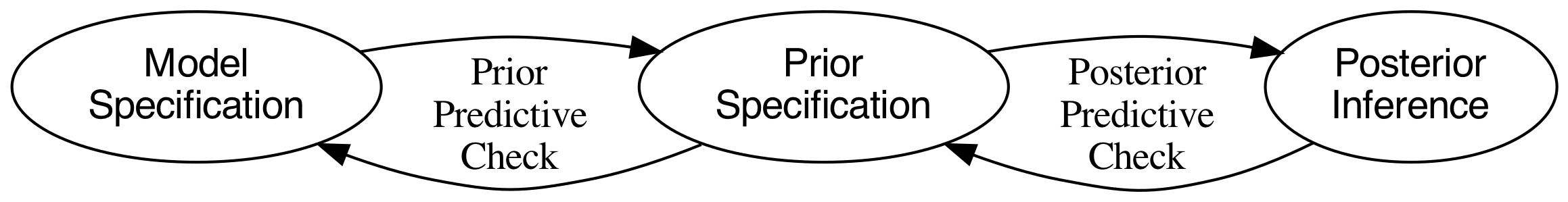
Predictive checks are a great way to validate a model. The idea is to generate data from the model using parameters from draws from the prior or posterior. Prior predictive check is when we simulate data using model parameter values drawn from the prior distribution, and posterior predictive check is is when we simulate data using model parameter values drawn from the posterior distribution.

The workflow we do when specifying and sampling Bayesian models is not linear or acyclic (Gelman et al., 2020). This means that we need to iterate several times between the different stages in order to find a model that captures best the data generating process with the desired assumptions. The figure below demonstrates the workflow ^[3].

This is quite easy in Turing. Our six-sided dice model already has a posterior distribution which is the object chain. We need to create a prior distribution for our model. To accomplish this, instead of supplying a MCMC sampler like NUTS(), we supply the "sampler" Prior() inside Turing's sample() function:

prior_chain = sample(model, Prior(), 2_000);

Now we can perform predictive checks using both the prior (prior_chain) or posterior (chain) distributions. To draw from the prior and posterior predictive distributions we instantiate a "predictive model", i.e. a Turing model but with the observations set to missing, and then calling predict() on the predictive model and the previously drawn samples. First let's do the prior predictive check:

missing_data = similar(my_data, Missing) # vector of `missing`
model_missing = dice_throw(missing_data) # instantiate the "predictive model
prior_check = predict(model_missing, prior_chain);

Here we are creating a missing_data object which is a Vector of the same length as the my_data and populated with type missing as values. We then instantiate a new dice_throw model with the missing_data vector as the y argument. Finally, we call predict() on the predictive model and the previously drawn samples, which in our case are the samples from the prior distribution (prior_chain).

Note that predict() returns a Chains object from MCMCChains.jl:

typeof(prior_check)

MCMCChains.Chains{Float64, AxisArrays.AxisArray{Float64, 3, Array{Float64, 3}, Tuple{AxisArrays.Axis{:iter, StepRange{Int64, Int64}}, AxisArrays.Axis{:var, Vector{Symbol}}, AxisArrays.Axis{:chain, UnitRange{Int64}}}}, Missing, @NamedTuple{parameters::Vector{Symbol}, internals::Vector{Symbol}}, @NamedTuple{varname_to_symbol::OrderedCollections.OrderedDict{AbstractPPL.VarName, Symbol}}}

And we can call summarystats():

summarystats(prior_check[:, 1:5, :]) # just the first 5 prior samples

Summary Statistics
  parameters      mean       std      mcse    ess_bulk   ess_tail      rhat   ess_per_sec
      Symbol   Float64   Float64   Float64     Float64    Float64   Float64       Missing

        y[1]    3.4265    1.7433    0.0396   1966.1989        NaN    1.0016       missing
        y[2]    3.4815    1.6974    0.0414   1672.3452        NaN    1.0024       missing
        y[3]    3.4620    1.7149    0.0396   1878.7524        NaN    1.0022       missing
        y[4]    3.4905    1.7177    0.0387   1960.3938        NaN    1.0006       missing
        y[5]    3.5095    1.7101    0.0386   2002.7276        NaN    0.9998       missing

We can do the same with chain for a posterior predictive check:

posterior_check = predict(model_missing, chain);
summarystats(posterior_check[:, 1:5, :]) # just the first 5 posterior samples

Summary Statistics
  parameters      mean       std      mcse    ess_bulk   ess_tail      rhat   ess_per_sec
      Symbol   Float64   Float64   Float64     Float64    Float64   Float64       Missing

        y[1]    3.8050    1.6637    0.0510   1065.1417        NaN    0.9992       missing
        y[2]    3.6280    1.6638    0.0583    773.8349        NaN    1.0000       missing
        y[3]    3.6430    1.7007    0.0554    921.8019        NaN    1.0044       missing
        y[4]    3.5720    1.6845    0.0518   1052.7732        NaN    0.9993       missing
        y[5]    3.6390    1.7400    0.0546    988.2165        NaN    1.0012       missing

Conclusion

This is the basic overview of Turing usage. I hope that I could show you how simple and intuitive is to specify probabilistic models using Turing. First, specify a model with the macro @model, then sample from it by specifying the data, sampler and number of interactions. All probabilistic parameters (the ones that you've specified using ~) will be inferred with a full posterior density. Finally, you inspect the parameters' statistics like mean and standard deviation, along with convergence diagnostics like r_hat. Conveniently, you can plot stuff easily if you want to. You can also do predictive checks using either the posterior or prior model's distributions.

Footnotes

[1]	see 5. Markov Chain Monte Carlo (MCMC).

[2]	we'll cover those plots and diagnostics in 5. Markov Chain Monte Carlo (MCMC).

[3]	note that this workflow is a extremely simplified adaptation from the original workflow on which it was based. I suggest the reader to consult the original workflow of Gelman et al. (2020).

References

Ge, H., Xu, K., & Ghahramani, Z. (2018). Turing: A Language for Flexible Probabilistic Inference. International Conference on Artificial Intelligence and Statistics, 1682–1690. http://proceedings.mlr.press/v84/ge18b.html

Gelman, A., Vehtari, A., Simpson, D., Margossian, C. C., Carpenter, B., Yao, Y., … Modr’ak, M. (2020, November 3). Bayesian Workflow. Retrieved February 4, 2021, from http://arxiv.org/abs/2011.01808

Hardesty (2015). "Probabilistic programming does in 50 lines of code what used to take thousands". phys.org. April 13, 2015. Retrieved April 13, 2015. https://phys.org/news/2015-04-probabilistic-lines-code-thousands.html

Hoffman, M. D., & Gelman, A. (2011). The No-U-Turn Sampler: Adaptively Setting Path Lengths in Hamiltonian Monte Carlo. Journal of Machine Learning Research, 15(1), 1593–1623. Retrieved from http://arxiv.org/abs/1111.4246

Tarek, M., Xu, K., Trapp, M., Ge, H., & Ghahramani, Z. (2020). DynamicPPL: Stan-like Speed for Dynamic Probabilistic Models. ArXiv:2002.02702 [Cs, Stat]. http://arxiv.org/abs/2002.02702

Xu, K., Ge, H., Tebbutt, W., Tarek, M., Trapp, M., & Ghahramani, Z. (2020). AdvancedHMC.jl: A robust, modular and efficient implementation of advanced HMC algorithms. Symposium on Advances in Approximate Bayesian Inference, 1–10. http://proceedings.mlr.press/v118/xu20a.html