Multilevel Models (a.k.a. Hierarchical Models)

Bayesian hierarchical models (also called multilevel models) are a statistical model written at multiple levels (hierarchical form) that estimates the parameters of the posterior distribution using the Bayesian approach. The sub-models combine to form the hierarchical model, and Bayes' theorem is used to integrate them with the observed data and to account for all the uncertainty that is present. The result of this integration is the posterior distribution, also known as an updated probability estimate, as additional evidence of the likelihood function is integrated together with the prior distribution of the parameters.

Hierarchical modeling is used when information is available at several different levels of observation units. The hierarchical form of analysis and organization helps to understand multiparameter problems and also plays an important role in the development of computational strategies.

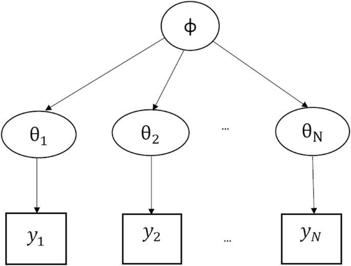
Hierarchical models are mathematical statements that involve several parameters, so that the estimates of some parameters depend significantly on the values of other parameters. The figure below shows a hierarchical model in which there is a $\phi$ hyperparameter that parameterizes the parameters $\theta_1, \theta_2, \dots, \theta_N$ that are finally used to infer the posterior density of some variable of interest $\mathbf{y} = y_1, y_2, \dots, y_N$.

When to use Multilevel Models?

Multilevel models are particularly suitable for research projects where participant data is organized at more than one level, i.e. nested data. Units of analysis are usually individuals (at a lower level) that are nested in contextual/aggregate units (at a higher level). An example is when we are measuring the performance of individuals and we have additional information about belonging to different groups such as sex, age group, hierarchical level, educational level or housing status.

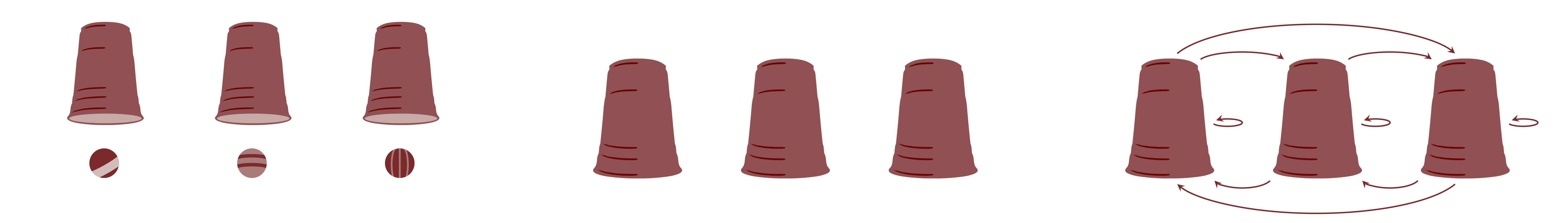
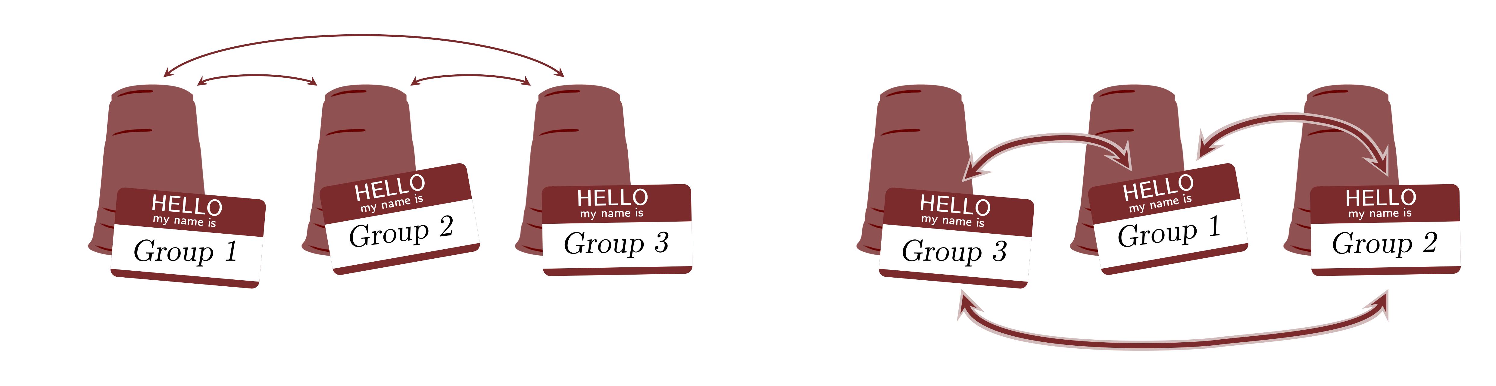
There is a main assumption that cannot be violated in multilevel models which is exchangeability (de Finetti, 1974; Nau, 2001). Yes, this is the same assumption that we discussed in 2. What is Bayesian Statistics?. This assumption assumes that groups are exchangeable. The figure below shows a graphical representation of the exchangeability. The groups shown as "cups" that contain observations shown as "balls". If in the model's inferences, this assumption is violated, then multilevel models are not appropriate. This means that, since there is no theoretical justification to support exchangeability, the inferences of the multilevel model are not robust and the model can suffer from several pathologies and should not be used for any scientific or applied analysis.

Hyperpriors

As the priors of the parameters are sampled from another prior of the hyperparameter (upper-level's parameter), which are called hyperpriors. This makes one group's estimates help the model to better estimate the other groups by providing more robust and stable estimates.

We call the global parameters as population effects (or population-level effects, also sometimes called fixed effects) and the parameters of each group as group effects (or group-level effects, also sometimes called random effects). That is why multilevel models are also known as mixed models in which we have both fixed effects and random effects.

Three Approaches to Multilevel Models

Multilevel models generally fall into three approaches:

1. Random-intercept model: each group receives a different intercept in addition to the global intercept.

2. Random-slope model: each group receives different coefficients for each (or a subset of) independent variable(s) in addition to a global intercept.

3. Random-intercept-slope model: each group receives both a different intercept and different coefficients for each independent variable in addition to a global intercept.

Random-Intercept Model

The first approach is the random-intercept model in which we specify a different intercept for each group, in addition to the global intercept. These group-level intercepts are sampled from a hyperprior.

To illustrate a multilevel model, I will use the linear regression example with a Gaussian/normal likelihood function. Mathematically a Bayesian multilevel random-slope linear regression model is:

$$\begin{aligned} \mathbf{y} &\sim \text{Normal}\left( \alpha + \alpha_j + \mathbf{X} \cdot \boldsymbol{\beta}, \sigma \right) \\ \alpha &\sim \text{Normal}(\mu_\alpha, \sigma_\alpha) \\ \alpha_j &\sim \text{Normal}(0, \tau) \\ \boldsymbol{\beta} &\sim \text{Normal}(\mu_{\boldsymbol{\beta}}, \sigma_{\boldsymbol{\beta}}) \\ \tau &\sim \text{Cauchy}^+(0, \psi_{\alpha})\\ \sigma &\sim \text{Exponential}(\lambda_\sigma) \end{aligned}$$

The priors on the global intercept $\alpha$, global coefficients $\boldsymbol{\beta}$ and error $\sigma$, along with the Gaussian/normal likelihood on $\mathbf{y}$ are the same as in the linear regression model. But now we have new parameters. The first are the group intercepts prior $\alpha_j$ that denotes that every group $1, 2, \dots, J$ has its own intercept sampled from a normal distribution centered on 0 with a standard deviation $\psi_\alpha$. This group intercept is added to the linear predictor inside the Gaussian/normal likelihood function. The group intercepts' standard deviation $\tau$ have a hyperprior (being a prior of a prior) which is sampled from a positive-constrained Cauchy distribution (a special case of the Student-$t$ distribution with degrees of freedom $\nu = 1$) with mean 0 and standard deviation $\sigma_\alpha$. This makes the group-level intercept's dispersions being sampled from the same parameter $\tau$ which allows the model to use information from one group intercept to infer robust information regarding another group's intercept dispersion and so on.

This is easily accomplished with Turing:

using Turing
using LinearAlgebra: I
using Statistics: mean, std
using Random: seed!
seed!(123)

@model function varying_intercept(
    X, idx, y; n_gr=length(unique(idx)), predictors=size(X, 2)
)
    #priors
    α ~ Normal(mean(y), 2.5 * std(y))       # population-level intercept
    β ~ filldist(Normal(0, 2), predictors)  # population-level coefficients
    σ ~ Exponential(std(y))                 # residual SD
    #prior for variance of random intercepts
    #usually requires thoughtful specification
    τ ~ truncated(Cauchy(0, 2); lower=0)    # group-level SDs intercepts
    αⱼ ~ filldist(Normal(0, τ), n_gr)       # group-level intercepts

    #likelihood
    ŷ = α .+ X * β .+ αⱼ[idx]
    return y ~ MvNormal(ŷ, σ^2 * I)
end;

Random-Slope Model

The second approach is the random-slope model in which we specify a different slope for each group, in addition to the global intercept. These group-level slopes are sampled from a hyperprior.

To illustrate a multilevel model, I will use the linear regression example with a Gaussian/normal likelihood function. Mathematically a Bayesian multilevel random-slope linear regression model is:

$$\begin{aligned} \mathbf{y} &\sim \text{Normal}\left( \alpha + \mathbf{X} \cdot \boldsymbol{\beta}_j \cdot \boldsymbol{\tau}, \sigma \right) \\ \alpha &\sim \text{Normal}(\mu_\alpha, \sigma_\alpha) \\ \boldsymbol{\beta}_j &\sim \text{Normal}(0, 1) \\ \boldsymbol{\tau} &\sim \text{Cauchy}^+(0, \psi_{\boldsymbol{\beta}})\\ \sigma &\sim \text{Exponential}(\lambda_\sigma) \end{aligned}$$

Here we have a similar situation from before with the same hyperprior, but now it is a hyperprior for the the group coefficients' standard deviation prior: $\boldsymbol{\beta}_j$. This makes the group-level coefficients's dispersions being sampled from the same parameter $\tau$ which allows the model to use information from one group coefficients to infer robust information regarding another group's coefficients dispersion and so on.

In Turing we can accomplish this as:

@model function varying_slope(X, idx, y; n_gr=length(unique(idx)), predictors=size(X, 2))
    #priors
    α ~ Normal(mean(y), 2.5 * std(y))                    # population-level intercept
    σ ~ Exponential(std(y))                              # residual SD
    #prior for variance of random slopes
    #usually requires thoughtful specification
    τ ~ filldist(truncated(Cauchy(0, 2); lower=0), n_gr) # group-level slopes SDs
    βⱼ ~ filldist(Normal(0, 1), predictors, n_gr)        # group-level standard normal slopes

    #likelihood
    ŷ = α .+ X * βⱼ * τ
    return y ~ MvNormal(ŷ, σ^2 * I)
end;

Random-Intercept-Slope Model

The third approach is the random-intercept-slope model in which we specify a different intercept and slope for each group, in addition to the global intercept. These group-level intercepts and slopes are sampled from hyperpriors.

To illustrate a multilevel model, I will use the linear regression example with a Gaussian/normal likelihood function. Mathematically a Bayesian multilevel random-intercept-slope linear regression model is:

$$\begin{aligned} \mathbf{y} &\sim \text{Normal}\left( \alpha + \alpha_j + \mathbf{X} \cdot \boldsymbol{\beta}_j \cdot \boldsymbol{\tau}_{\boldsymbol{\beta}}, \sigma \right) \\ \alpha &\sim \text{Normal}(\mu_\alpha, \sigma_\alpha) \\ \alpha_j &\sim \text{Normal}(0, \tau_{\alpha}) \\ \boldsymbol{\beta}_j &\sim \text{Normal}(0, 1) \\ \tau_{\alpha} &\sim \text{Cauchy}^+(0, \psi_{\alpha})\\ \boldsymbol{\tau}_{\boldsymbol{\beta}} &\sim \text{Cauchy}^+(0, \psi_{\boldsymbol{\beta}})\\ \sigma &\sim \text{Exponential}(\lambda_\sigma) \end{aligned}$$

Here we have a similar situation from before with the same hyperpriors, but now we fused both random-intercept and random-slope together.

In Turing we can accomplish this as:

@model function varying_intercept_slope(
    X, idx, y; n_gr=length(unique(idx)), predictors=size(X, 2)
)
    #priors
    α ~ Normal(mean(y), 2.5 * std(y))                     # population-level intercept
    σ ~ Exponential(std(y))                               # residual SD
    #prior for variance of random intercepts and slopes
    #usually requires thoughtful specification
    τₐ ~ truncated(Cauchy(0, 2); lower=0)                 # group-level SDs intercepts
    τᵦ ~ filldist(truncated(Cauchy(0, 2); lower=0), n_gr) # group-level slopes SDs
    αⱼ ~ filldist(Normal(0, τₐ), n_gr)                    # group-level intercepts
    βⱼ ~ filldist(Normal(0, 1), predictors, n_gr)         # group-level standard normal slopes

    #likelihood
    ŷ = α .+ αⱼ[idx] .+ X * βⱼ * τᵦ
    return y ~ MvNormal(ŷ, σ^2 * I)
end;

In all of the models, we are using the MvNormal construction where we specify both a vector of means (first positional argument) and a covariance matrix (second positional argument). Regarding the covariance matrix σ^2 * I, it uses the model's errors σ, here parameterized as a standard deviation, squares it to produce a variance paramaterization, and multiplies by I, which is Julia's LinearAlgebra standard module implementation to represent an identity matrix of any size.

Example - Cheese Ratings

For our example, I will use a famous dataset called cheese (Boatwright, McCulloch & Rossi, 1999), which is data from cheese ratings. A group of 10 rural and 10 urban raters rated 4 types of different cheeses (A, B, C and D) in two samples. So we have $4 \cdot 20 \cdot2 = 160$ observations and 4 variables:

• cheese: type of cheese from A to D

• rater: id of the rater from 1 to 10

• background: type of rater, either rural or urban

• y: rating of the cheese

Ok let's read our data with CSV.jl and output into a DataFrame from DataFrames.jl:

using DataFrames
using CSV
using HTTP

url = "https://raw.githubusercontent.com/storopoli/Bayesian-Julia/master/datasets/cheese.csv"
cheese = CSV.read(HTTP.get(url).body, DataFrame)
describe(cheese)

4×7 DataFrame
 Row │ variable    mean     min    median  max    nmissing  eltype
     │ Symbol      Union…   Any    Union…  Any    Int64     DataType
─────┼───────────────────────────────────────────────────────────────
   1 │ cheese               A              D             0  String1
   2 │ rater       5.5      1      5.5     10            0  Int64
   3 │ background           rural          urban         0  String7
   4 │ y           70.8438  33     71.5    91            0  Int64

As you can see from the describe() output, the mean cheese ratings is around 70 ranging from 33 to 91.

In order to prepare the data for Turing, I will convert the Strings in variables cheese and background to Ints. Regarding cheese, I will create 4 dummy variables one for each cheese type; and background will be converted to integer data taking two values: one for each background type. My intent is to model background as a group both for intercept and coefficients. Take a look at how the data will look like for the first 5 observations:

for c in unique(cheese[:, :cheese])
    cheese[:, "cheese_$c"] = ifelse.(cheese[:, :cheese] .== c, 1, 0)
end

cheese[:, :background_int] = map(cheese[:, :background]) do b
    if b == "rural"
        1
    elseif b == "urban"
        2
    else
        missing
    end
end

first(cheese, 5)

5×9 DataFrame
 Row │ cheese   rater  background  y      cheese_A  cheese_B  cheese_C  cheese_D  background_int
     │ String1  Int64  String7     Int64  Int64     Int64     Int64     Int64     Int64
─────┼───────────────────────────────────────────────────────────────────────────────────────────
   1 │ A            1  rural          67         1         0         0         0               1
   2 │ A            1  rural          66         1         0         0         0               1
   3 │ B            1  rural          51         0         1         0         0               1
   4 │ B            1  rural          53         0         1         0         0               1
   5 │ C            1  rural          75         0         0         1         0               1

Now let's us instantiate our model with the data. Here, I will specify a vector of Ints named idx to represent the different observations' group memberships. This will be used by Turing when we index a parameter with the idx, e.g. αⱼ[idx].

X = Matrix(select(cheese, Between(:cheese_A, :cheese_D)));
y = cheese[:, :y];
idx = cheese[:, :background_int];

The first model is the varying_intercept:

model_intercept = varying_intercept(X, idx, y)
chain_intercept = sample(model_intercept, NUTS(), MCMCThreads(), 1_000, 4)
println(DataFrame(summarystats(chain_intercept)))

9×8 DataFrame
 Row │ parameters  mean       std       naive_se   mcse        ess       rhat     ess_per_sec
     │ Symbol      Float64    Float64   Float64    Float64     Float64   Float64  Float64
─────┼────────────────────────────────────────────────────────────────────────────────────────
   1 │ α            71.0623   5.20909   0.0823629  0.207975     614.756  1.01148      21.0699
   2 │ β[1]          2.92058  1.34748   0.0213055  0.0273105   2229.83   1.00032      76.4242
   3 │ β[2]        -10.6231   1.41028   0.0222985  0.0293236   2165.45   1.00098      74.2175
   4 │ β[3]          6.54211  1.33203   0.0210612  0.0231375   2059.77   1.00089      70.5957
   5 │ β[4]          1.08986  1.33386   0.0210901  0.0245427   2191.31   1.00158      75.1039
   6 │ σ             7.39302  0.454211  0.0071817  0.00765719  2836.78   1.00025      97.2266
   7 │ τ             6.35652  6.22258   0.0983876  0.212702     854.35   1.00035      29.2816
   8 │ αⱼ[1]        -3.73622  5.16514   0.081668   0.206153     623.412  1.01241      21.3666
   9 │ αⱼ[2]         3.3567   5.12434   0.0810229  0.199044     655.616  1.01115      22.4703

Here we can see that the model has a population-level intercept α along with population-level coefficients βs for each cheese dummy variable. But notice that we have also group-level intercepts for each of the groups αⱼs. Specifically, αⱼ[1] are the rural raters and αⱼ[2] are the urban raters.

Now let's go to the second model, varying_slope:

model_slope = varying_slope(X, idx, y)
chain_slope = sample(model_slope, NUTS(), MCMCThreads(), 1_000, 4)
println(DataFrame(summarystats(chain_slope)))

12×8 DataFrame
 Row │ parameters  mean        std       naive_se    mcse        ess       rhat      ess_per_sec
     │ Symbol      Float64     Float64   Float64     Float64     Float64   Float64   Float64
─────┼───────────────────────────────────────────────────────────────────────────────────────────
   1 │ α           70.9545     5.07773   0.0802859   0.143448     894.061  1.00292      21.7809
   2 │ σ            7.99234    0.44656   0.00706073  0.00835223  3407.51   1.00007      83.0127
   3 │ τ[1]         6.34027    5.63494   0.0890963   0.274731     239.735  1.02104       5.84035
   4 │ τ[2]         5.98939    5.06917   0.0801506   0.204766     696.528  1.0077       16.9686
   5 │ βⱼ[1,1]      0.2465     0.809372  0.0127973   0.0156597   1955.67   1.00037      47.6434
   6 │ βⱼ[2,1]     -0.914336   1.05018   0.0166048   0.0352163   1033.32   1.00451      25.1734
   7 │ βⱼ[3,1]      0.5831     0.906283  0.0143296   0.025254    1430.21   1.00043      34.8424
   8 │ βⱼ[4,1]      0.0899121  0.791636  0.0125169   0.0158593   2072.59   1.00055      50.4918
   9 │ βⱼ[1,2]      0.228278   0.807897  0.012774    0.0190118   1538.33   1.00194      37.4763
  10 │ βⱼ[2,2]     -0.917557   1.039     0.0164281   0.0341002    914.133  1.00275      22.2699
  11 │ βⱼ[3,2]      0.57743    0.921847  0.0145757   0.0293906   1128.26   1.00147      27.4865
  12 │ βⱼ[4,2]      0.0979169  0.806051  0.0127448   0.0162976   1810.83   0.999819     44.1149

Here we can see that the model has still a population-level intercept α. But now our population-level coefficients βs are replaced by group-level coefficients βⱼs along with their standard deviation τᵦs. Specifically βⱼ's first index denotes the 4 dummy cheese variables' and the second index are the group membership. So, for example βⱼ[1,1] is the coefficient for cheese_A and rural raters (group 1).

Now let's go to the third model, varying_intercept_slope:

model_intercept_slope = varying_intercept_slope(X, idx, y)
chain_intercept_slope = sample(model_intercept_slope, NUTS(), MCMCThreads(), 1_000, 4)
println(DataFrame(summarystats(chain_intercept_slope)))

15×8 DataFrame
 Row │ parameters  mean        std       naive_se    mcse       ess        rhat     ess_per_sec
     │ Symbol      Float64     Float64   Float64     Float64    Float64    Float64  Float64
─────┼──────────────────────────────────────────────────────────────────────────────────────────
   1 │ α           69.264      9.28582   0.146822    0.821065     19.0963  1.32241     0.282955
   2 │ σ            7.00827    0.40295   0.00637119  0.0216265    57.0466  1.08995     0.845273
   3 │ τₐ           6.05739    5.10782   0.0807618   0.206374    631.418   1.01922     9.35587
   4 │ τᵦ[1]        7.76514    6.13411   0.0969888   0.486895     51.7597  1.08319     0.766936
   5 │ τᵦ[2]        5.06397    4.9826    0.0787819   0.317945     59.0281  1.08867     0.874633
   6 │ αⱼ[1]       -3.93082    5.35868   0.0847282   0.244448    458.558   1.00976     6.79457
   7 │ αⱼ[2]        3.24853    5.36536   0.0848338   0.232919    468.668   1.01077     6.94436
   8 │ βⱼ[1,1]      0.419978   0.855047  0.0135195   0.0605762    31.2381  1.17063     0.462862
   9 │ βⱼ[2,1]     -0.805084   1.04746   0.0165618   0.0561349    76.9592  1.07045     1.14032
  10 │ βⱼ[3,1]      0.73379    0.917971  0.0145144   0.0645445    33.0845  1.15978     0.490221
  11 │ βⱼ[4,1]      0.249376   0.824109  0.0130303   0.0554565    32.5471  1.16532     0.482258
  12 │ βⱼ[1,2]      0.214857   0.733133  0.0115919   0.0247082  1007.64    1.00338    14.9305
  13 │ βⱼ[2,2]     -0.587502   1.21115   0.0191499   0.100328     22.1007  1.25767     0.327471
  14 │ βⱼ[3,2]      0.473844   0.840948  0.0132966   0.0377764   305.282   1.01906     4.52343
  15 │ βⱼ[4,2]     -0.0235769  0.811298  0.0128277   0.0424477    86.109   1.05794     1.2759

Now we have fused the previous model in one. We still have a population-level intercept α. But now we have in the same model group-level intercepts for each of the groups αⱼs and group-level along with their standard deviation τₐ. We also have the coefficients βⱼs with their standard deviation τᵦs. The parameters are interpreted exactly as the previous cases.

References

Boatwright, P., McCulloch, R., & Rossi, P. (1999). Account-level modeling for trade promotion: An application of a constrained parameter hierarchical model. Journal of the American Statistical Association, 94(448), 1063–1073.

de Finetti, B. (1974). Theory of Probability (Volume 1). New York: John Wiley & Sons.

Nau, R. F. (2001). De Finetti was Right: Probability Does Not Exist. Theory and Decision, 51(2), 89–124. https://doi.org/10.1023/A:1015525808214