Bonus: Epidemiological Models using ODE Solvers in Turing
Ok, now this is something that really makes me very excited with Julia's ecosystem. If you want to use an Ordinary Differential Equation solver in your Turing model, you don't need to code it from scratch. You've just borrow a pre-made one from DifferentialEquations.jl. This is what makes Julia so great. We can use functions and types defined in other packages into another package and it will probably work either straight out of the bat or without much effort!
For this tutorial I'll be using Brazil's COVID data from the Media Consortium. For reproducibility, we'll restrict the data to the year of 2020:
using Downloads
using DataFrames
using CSV
using Chain
using Dates

url = "https://data.brasil.io/dataset/covid19/caso_full.csv.gz"
file = Downloads.download(url)
df = DataFrame(CSV.File(file))
br = @chain df begin
    filter(
        [:date, :city] =>
            (date, city) ->
                date < Dates.Date("2021-01-01") &&
                    date > Dates.Date("2020-04-01") &&
                    ismissing(city),
        _,
    )
    groupby(:date)
    combine(
        [
            :estimated_population_2019,
            :last_available_confirmed_per_100k_inhabitants,
            :last_available_deaths,
            :new_confirmed,
            :new_deaths,
        ] .=>
            sum .=> [
                :estimated_population_2019,
                :last_available_confirmed_per_100k_inhabitants,
                :last_available_deaths,
                :new_confirmed,
                :new_deaths,
            ],
    )
end;
Let's take a look in the first observations
first(br, 5)5×6 DataFrame
Row │ date estimated_population_2019 last_available_confirmed_per_100k_inhabitants last_available_deaths new_confirmed new_deaths
│ Date Int64 Float64 Int64 Int64 Int64
─────┼────────────────────────────────────────────────────────────────────────────────────────────────────────────────────────────────────────
1 │ 2020-04-02 210147125 79.6116 305 1167 61
2 │ 2020-04-03 210147125 90.9596 365 1114 60
3 │ 2020-04-04 210147125 103.622 445 1169 80
4 │ 2020-04-05 210147125 115.594 496 1040 51
5 │ 2020-04-06 210147125 125.766 569 840 73Also the bottom rows
last(br, 5)5×6 DataFrame
Row │ date estimated_population_2019 last_available_confirmed_per_100k_inhabitants last_available_deaths new_confirmed new_deaths
│ Date Int64 Float64 Int64 Int64 Int64
─────┼────────────────────────────────────────────────────────────────────────────────────────────────────────────────────────────────────────
1 │ 2020-12-27 210147125 1.22953e5 191250 17614 337
2 │ 2020-12-28 210147125 1.23554e5 191788 27437 538
3 │ 2020-12-29 210147125 1.24291e5 192839 56371 1051
4 │ 2020-12-30 210147125 1.25047e5 194056 55600 1217
5 │ 2020-12-31 210147125 1.25724e5 195072 54469 1016Here is a plot of the data:
using AlgebraOfGraphics
using CairoMakie
f = Figure()
plt = data(br) * mapping(:date => L"t", :new_confirmed => "infected daily") * visual(Lines)
draw!(f[1, 1], plt)
The Susceptible-Infected-Recovered (SIR) (Grinsztajn, Semenova, Margossian & Riou, 2021) model splits the population in three time-dependent compartments: the susceptible, the infected (and infectious), and the recovered (and not infectious) compartments. When a susceptible individual comes into contact with an infectious individual, the former can become infected for some time, and then recover and become immune. The dynamics can be summarized in a system ODEs:
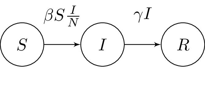
where:
– the number of people susceptible to becoming infected (no immunity)
– the number of people currently infected (and infectious)
– the number of recovered people (we assume they remain immune indefinitely)
– the constant rate of infectious contact between people
– constant recovery rate of infected individuals
How to code an ODE in Julia?
It's very easy:
Create a ODE function
Choose:
Initial Conditions –
Parameters –
Time Span –
Optional – Solver or leave blank for auto
PS: If you like SIR models checkout epirecipes/sir-julia
The following function provides the derivatives of the model, which it changes in-place. State variables and parameters are unpacked from u and p; this incurs a slight performance hit, but makes the equations much easier to read.
using DifferentialEquations

function sir_ode!(du, u, p, t)
    (S, I, R) = u
    (β, γ) = p
    N = S + I + R
    infection = β * I * S / N
    recovery = γ * I
    @inbounds begin
        du[1] = -infection # Susceptible
        du[2] = infection - recovery # Infected
        du[3] = recovery # Recovered
    end
    return nothing
end;
This is what the infection would look with some fixed β and γ in a timespan of 100 days starting from day one with 1,167 infected (Brazil in April 2020):
i₀ = first(br[:, :new_confirmed])
N = maximum(br[:, :estimated_population_2019])

u = [N - i₀, i₀, 0.0]
p = [0.5, 0.05]
prob = ODEProblem(sir_ode!, u, (1.0, 100.0), p)
sol_ode = solve(prob)
f = Figure()
plt =
    data(stack(DataFrame(sol_ode), Not(:timestamp))) *
    mapping(
        :timestamp => L"t",
        :value => L"N";
        color=:variable => renamer(["value1" => "S", "value2" => "I", "value3" => "R"]),
    ) *
    visual(Lines; linewidth=3)
draw!(f[1, 1], plt; axis=(; title="SIR Model for 100 days, β = $(p[1]), γ = $(p[2])"))
How to use a ODE solver in a Turing Model
Please note that we are using the alternative negative binomial parameterization as specified in 8. Bayesian Regression with Count Data:
function NegativeBinomial2(μ, ϕ)
    p = 1 / (1 + μ / ϕ)
    r = ϕ

    return NegativeBinomial(r, p)
end
NegativeBinomial2 (generic function with 1 method)Now this is the fun part. It's easy: just stick it inside!
using Turing
using LazyArrays
using Random: seed!
seed!(123)

@model function bayes_sir(infected, i₀, r₀, N)
    #calculate number of timepoints
    l = length(infected)

    #priors
    β ~ TruncatedNormal(2, 1, 1e-4, 10)     # using 10 because numerical issues arose
    γ ~ TruncatedNormal(0.4, 0.5, 1e-4, 10) # using 10 because numerical issues arose
    ϕ⁻ ~ truncated(Exponential(5); lower=0, upper=1e5)
    ϕ = 1.0 / ϕ⁻

    #ODE Stuff
    I = i₀
    u0 = [N - I, I, r₀] # S,I,R
    p = [β, γ]
    tspan = (1.0, float(l))
    prob = ODEProblem(sir_ode!, u0, tspan, p)
    sol = solve(
        prob,
        Tsit5(); # similar to Dormand-Prince RK45 in Stan but 20% faster
        saveat=1.0,
    )
    solᵢ = Array(sol)[2, :] # New Infected
    solᵢ = max.(1e-4, solᵢ) # numerical issues arose

    #likelihood
    return infected ~ arraydist(LazyArray(@~ NegativeBinomial2.(solᵢ, ϕ)))
end;
Now run the model and inspect our parameters estimates. We will be using the default NUTS() sampler with 1_000 samples on only one Markov chain:
infected = br[:, :new_confirmed]
r₀ = first(br[:, :new_deaths])
model_sir = bayes_sir(infected, i₀, r₀, N)
chain_sir = sample(model_sir, NUTS(), 1_000)
summarystats(chain_sir[[:β, :γ]])
Summary Statistics
parameters mean std mcse ess_bulk ess_tail rhat ess_per_sec
Symbol Float64 Float64 Float64 Float64 Float64 Float64 Float64
β 1.1199 0.0292 0.0013 477.2173 505.0551 0.9996 11.2615
γ 1.0869 0.0296 0.0014 477.1981 493.8323 0.9996 11.2610
Hope you had learned some new bayesian computational skills and also took notice of the amazing potential of Julia's ecosystem of packages.
References
Grinsztajn, L., Semenova, E., Margossian, C. C., & Riou, J. (2021). Bayesian workflow for disease transmission modeling in Stan. ArXiv:2006.02985 [q-Bio, Stat]. http://arxiv.org/abs/2006.02985