Markov Chain Monte Carlo (MCMC)
The main computational barrier for Bayesian statistics is the denominator of the Bayes formula:
In discrete cases we can turn the denominator into a sum of all parameters using the chain rule of probability:
This is also called marginalization:
However, in the continuous cases the denominator becomes a very large and complicated integral to calculate:
In many cases this integral becomes intractable (incalculable) and therefore we must find other ways to calculate the posterior probability in (1) without using the denominator .
What is the denominator for?
Quick answer: to normalize the posterior in order to make it a valid probability distribution. This means that the sum of all probabilities of the possible events in the probability distribution must be equal to 1:
in the case of discrete probability distribution:
in the case of continuous probability distribution:
What if we remove this denominator?
When we remove the denominator we have that the posterior is proportional to the prior multiplied by the likelihood [1].
This YouTube video explains the denominator problem very well, see below:
Markov Chain Monte Carlo (MCMC)
This is where Markov Chain Monte Carlo comes in. MCMC is a broad class of computational tools for approximating integrals and generating samples from a posterior probability (Brooks, Gelman, Jones & Meng, 2011). MCMC is used when it is not possible to sample directly from the subsequent probabilistic distribution . Instead, we sample in an iterative manner such that at each step of the process we expect the distribution from which we sample (here means simulated) becomes increasingly similar to the posterior . All of this is to eliminate the (often impossible) calculation of the denominator .
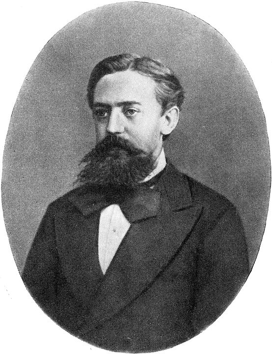
The idea is to define an ergodic Markov chain (that is to say that there is a single stationary distribution) of which the set of possible states is the sample space and the stationary distribution is the distribution to be approximated (or sampled). Let be a simulation of the chain. The Markov chain converges to the stationary distribution of any initial state after a large enough number of iterations , the distribution of the state will be similar to the stationary distribution, so we can use it as a sample. Markov chains have a property that the probability distribution of the next state depends only on the current state and not on the sequence of events that preceded: . This property is called Markovian, after the mathematician Andrey Markov (see figure below). Similarly, repeating this argument with as the starting point, we can use as a sample, and so on. We can then use the state sequence as almost independent samples of the stationary distribution of the Markov chain.
The effectiveness of this approach depends on:
how big must be to ensure a suitably good sample; and
computational power required for each iteration of the Markov chain.
In addition, it is customary to discard the first iterations of the algorithm as they are usually not representative of the distribution to be approximated. In the initial iterations of MCMC algorithms, generally the Markov current is in a warm-up process[2] and its state is far from ideal to start a reliable sampling. It is generally recommended to discard half of the iterations (Gelman, Carlin, Stern, Dunson, Vehtari, & Rubin, 2013a). For example: if the Markov chain has 4,000 iterations, we discard the first 2,000 as warm-up.
Monte Carlo Method
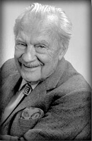
Stanislaw Ulam (figure below), who participated in the Manhattan project and when trying to calculate the neutron diffusion process for the hydrogen bomb ended up creating a class of methods called Monte Carlo.
Monte Carlo methods have the underlying concept of using randomness to solve problems that can be deterministic in principle. They are often used in physical and mathematical problems and are most useful when it is difficult or impossible to use other approaches. Monte Carlo methods are used mainly in three classes of problems: optimization, numerical integration and generating sample from a probability distribution.
The idea for the method came to Ulam while playing solitaire during his recovery from surgery, as he thought about playing hundreds of games to statistically estimate the probability of a successful outcome. As he himself mentions in Eckhardt (1987):
"The first thoughts and attempts I made to practice [the Monte Carlo method] were suggested by a question which occurred to me in 1946 as I was convalescing from an illness and playing solitaires. The question was what are the chances that a Canfield solitaire laid out with 52 cards will come out successfully? After spending a lot of time trying to estimate them by pure combinatorial calculations, I wondered whether a more practical method than "abstract thinking" might not be to lay it out say one hundred times and simply observe and count the number of successful plays. This was already possible to envisage with the beginning of the new era of fast computers, and I immediately thought of problems of neutron diffusion and other questions of mathematical physics, and more generally how to change processes described by certain differential equations into an equivalent form interpretable as a succession of random operations. Later... [in 1946, I ] described the idea to John von Neumann and we began to plan actual calculations."
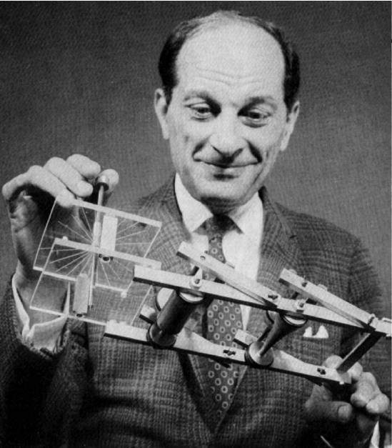
Because it was secret, von Neumann and Ulam's work required a codename. A colleague of von Neumann and Ulam, Nicholas Metropolis (figure below), suggested using the name "Monte Carlo", which refers to Casino Monte Carlo in Monaco, where Ulam's uncle (Michał Ulam) borrowed money from relatives to gamble.
The applications of the Monte Carlo method are numerous: physical sciences, engineering, climate change, computational biology, computer graphics, applied statistics, artificial intelligence, search and rescue, finance and business and law. In the scope of these tutorials we will focus on applied statistics and specifically in the context of Bayesian inference: providing a random sample of the posterior distribution.
Simulations
I will do some simulations to illustrate MCMC algorithms and techniques. So, here's the initial setup:
using CairoMakie
using Distributions
using Random

Random.seed!(123);
Let's start with a toy problem of a multivariate normal distribution of and , where
If we assign and (mean 0 and standard deviation 1 for both and ), we have the following formulation from (6):
All that remains is to assign a value for in (7) for the correlation between and . For our example we will use correlation of 0.8 ():
const N = 100_000
const μ = [0, 0]
const Σ = [1 0.8; 0.8 1]

const mvnormal = MvNormal(μ, Σ)
FullNormal(
dim: 2
μ: [0.0, 0.0]
Σ: [1.0 0.8; 0.8 1.0]
)
In the figure below it is possible to see a contour plot of the PDF of a multivariate normal distribution composed of two normal variables and , both with mean 0 and standard deviation 1. The correlation between and is :
x = -3:0.01:3
y = -3:0.01:3
dens_mvnormal = [pdf(mvnormal, [i, j]) for i in x, j in y]
f, ax, c = contourf(x, y, dens_mvnormal; axis=(; xlabel=L"X", ylabel=L"Y"))
Colorbar(f[1, 2], c)
Also a surface plot can be seen below for you to get a 3-D intuition of what is going on:
f, ax, s = surface(
    x,
    y,
    dens_mvnormal;
    axis=(type=Axis3, xlabel=L"X", ylabel=L"Y", zlabel="PDF", azimuth=pi / 8),
)
Metropolis and Metropolis-Hastings
The first MCMC algorithm widely used to generate samples from Markov chain originated in physics in the 1950s (in a very close relationship with the atomic bomb at the Manhattan project) and is called Metropolis (Metropolis, Rosenbluth, Rosenbluth, Teller, & Teller, 1953) in honor of the first author Nicholas Metropolis (figure above). In summary, the Metropolis algorithm is an adaptation of a random walk with an acceptance/rejection rule to converge to the target distribution.
The Metropolis algorithm uses a proposal distribution ( stands for jumping distribution and indicates which state of the Markov chain we are in) to define next values of the distribution . This distribution must be symmetrical:
In the 1970s, a generalization of the Metropolis algorithm emerged that does not require that the proposal distributions be symmetric. The generalization was proposed by Wilfred Keith Hastings (Hastings, 1970) (figure below) and is called Metropolis-Hastings algorithm.

Metropolis Algorithm
The essence of the algorithm is a random walk through the parameters' sample space, where the probability of the Markov chain changing state is defined as:
This means that the Markov chain will only change to a new state under two conditions:
When the probability of the parameters proposed by the random walk is greater than the probability of the parameters of the current state , we change with 100% probability. Note that if then the function chooses the value 1 which means 100%.
When the probability of the parameters proposed by the random walk is less than the probability of the parameters of the current state , we changed with a probability equal to the proportion of that difference. Note that if then the function does not choose the value 1, but the value which equates the proportion of the probability of the proposed parameters to the probability of the parameters at the current state.
Anyway, at each iteration of the Metropolis algorithm, even if the Markov chain changes state or not, we sample the parameter anyway. That is, if the chain does not change to a new state, will be sampled twice (or more if the current is stationary in the same state).
The Metropolis-Hastings algorithm can be described in the following way [3] ( is the parameter, or set of parameters, of interest and is the data):
Define a starting point of which , or sample it from an initial distribution . can be a normal distribution or a prior distribution of ().
For :
Sample a proposed from a proposal distribution in time , .
Calculate the ratio of probabilities:
Metropolis:
Metropolis-Hastings:
Assign:
Limitations of the Metropolis Algorithm
The limitations of the Metropolis-Hastings algorithm are mainly computational. With randomly generated proposals, it usually takes a large number of iterations to enter areas of higher (more likely) posterior densities. Even efficient Metropolis-Hastings algorithms sometimes accept less than 25% of the proposals (Roberts, Gelman & Gilks, 1997). In lower-dimensional situations, the increased computational power can compensate for the lower efficiency to some extent. But in higher-dimensional and more complex modeling situations, bigger and faster computers alone are rarely enough to overcome the challenge.
Metropolis – Implementation
In our toy example we will assume that is symmetric, thus , so I'll just implement the Metropolis algorithm (not the Metropolis-Hastings algorithm).
Below I created a Metropolis sampler for our toy example. At the end it prints the acceptance rate of the proposals. Here I am using the same proposal distribution for both and : a uniform distribution parameterized with a width parameter:
I will use the already known Distributions.jl MvNormal from the plots above along with the logpdf() function to calculate the PDF of the proposed and current s. It is easier to work with probability logs than with the absolute values[4]. Mathematically we will compute:
Here is a simple implementation in Julia:
function metropolis(
    S::Int64,
    width::Float64,
    ρ::Float64;
    μ_x::Float64=0.0,
    μ_y::Float64=0.0,
    σ_x::Float64=1.0,
    σ_y::Float64=1.0,
    start_x=-2.5,
    start_y=2.5,
    seed=123,
)
    rgn = MersenneTwister(seed)
    binormal = MvNormal([μ_x; μ_y], [σ_x ρ; ρ σ_y])
    draws = Matrix{Float64}(undef, S, 2)
    accepted = 0::Int64
    x = start_x
    y = start_y
    @inbounds draws[1, :] = [x y]
    for s in 2:S
        x_ = rand(rgn, Uniform(x - width, x + width))
        y_ = rand(rgn, Uniform(y - width, y + width))
        r = exp(logpdf(binormal, [x_, y_]) - logpdf(binormal, [x, y]))

        if r > rand(rgn, Uniform())
            x = x_
            y = y_
            accepted += 1
        end
        @inbounds draws[s, :] = [x y]
    end
    println("Acceptance rate is: $(accepted / S)")
    return draws
end
metropolis (generic function with 1 method)Now let's run our metropolis() algorithm for the bivariate normal case with S = 10_000, width = 2.75 and ρ = 0.8:
const S = 10_000
const width = 2.75
const ρ = 0.8

X_met = metropolis(S, width, ρ);
Acceptance rate is: 0.2116
Take a quick peek into X_met, we'll see it's a matrix of and values as columns and the time as rows:
X_met[1:10, :]10×2 Matrix{Float64}:
-2.5 2.5
-2.5 2.5
-3.07501 1.47284
-2.60189 -0.990426
-2.60189 -0.990426
-0.592119 -0.34422
-0.592119 -0.34422
-0.592119 -0.34422
-0.592119 -0.34422
-0.592119 -0.34422Also note that the acceptance of the proposals was 21%, the expected for Metropolis algorithms (around 20-25%) (Roberts et. al, 1997).
We can construct Chains object using MCMCChains.jl[5] by passing a matrix along with the parameters names as symbols inside the Chains() constructor:
using MCMCChains

chain_met = Chains(X_met, [:X, :Y]);
Then we can get summary statistics regarding our Markov chain derived from the Metropolis algorithm:
summarystats(chain_met)Summary Statistics
parameters mean std mcse ess_bulk ess_tail rhat ess_per_sec
Symbol Float64 Float64 Float64 Float64 Float64 Float64 Missing
X -0.0314 0.9984 0.0313 1022.8896 1135.7248 0.9999 missing
Y -0.0334 0.9784 0.0305 1028.0976 1046.3325 0.9999 missing
Both of X and Y have mean close to 0 and standard deviation close to 1 (which are the theoretical values). Take notice of the ess (effective sample size - ESS) is approximate 1,000. So let's calculate the efficiency of our Metropolis algorithm by dividing the ESS by the number of sampling iterations that we've performed:
mean(summarystats(chain_met)[:, :ess_tail]) / S0.10910286584687137Our Metropolis algorithm has around 10.2% efficiency. Which, in my honest opinion, sucks...(😂)
Metropolis – Visual Intuition
I believe that a good visual intuition, even if you have not understood any mathematical formula, is the key for you to start a fruitful learning journey. So I made some animations!
The animation in figure below shows the first 100 simulations of the Metropolis algorithm used to generate X_met. Note that in several iterations the proposal is rejected and the algorithm samples the parameters and from the previous state (which becomes the current one, since the proposal is refused). The blue ellipsis represents the 90% HPD of our toy example's bivariate normal distribution.
Note: HPD stands for Highest Probability Density (which in our case the posterior's 90% probability range).
using LinearAlgebra: eigvals, eigvecs
#source: https://discourse.julialang.org/t/plot-ellipse-in-makie/82814/4
function getellipsepoints(cx, cy, rx, ry, θ)
    t = range(0, 2 * pi; length=100)
    ellipse_x_r = @. rx * cos(t)
    ellipse_y_r = @. ry * sin(t)
    R = [cos(θ) sin(θ); -sin(θ) cos(θ)]
    r_ellipse = [ellipse_x_r ellipse_y_r] * R
    x = @. cx + r_ellipse[:, 1]
    y = @. cy + r_ellipse[:, 2]
    return (x, y)
end
function getellipsepoints(μ, Σ; confidence=0.95)
    quant = sqrt(quantile(Chisq(2), confidence))
    cx = μ[1]
    cy = μ[2]

    egvs = eigvals(Σ)
    if egvs[1] > egvs[2]
        idxmax = 1
        largestegv = egvs[1]
        smallesttegv = egvs[2]
    else
        idxmax = 2
        largestegv = egvs[2]
        smallesttegv = egvs[1]
    end

    rx = quant * sqrt(largestegv)
    ry = quant * sqrt(smallesttegv)

    eigvecmax = eigvecs(Σ)[:, idxmax]
    θ = atan(eigvecmax[2] / eigvecmax[1])
    if θ < 0
        θ += 2 * π
    end

    return getellipsepoints(cx, cy, rx, ry, θ)
end

f, ax, l = lines(
    getellipsepoints(μ, Σ; confidence=0.9)...;
    label="90% HPD",
    linewidth=2,
    axis=(; limits=(-3, 3, -3, 3), xlabel=L"\theta_1", ylabel=L"\theta_2"),
)
axislegend(ax)
record(f, joinpath(@OUTPUT, "met_anim.gif"); framerate=5) do frame
    for i in 1:100
        scatter!(ax, (X_met[i, 1], X_met[i, 2]); color=(:red, 0.5))
        linesegments!(X_met[i:(i + 1), 1], X_met[i:(i + 1), 2]; color=(:green, 0.5))
        recordframe!(frame)
    end
end;
Now let's take a look how the first 1,000 simulations were, excluding 1,000 initial iterations as warm-up.
const warmup = 1_000

f, ax, l = lines(
    getellipsepoints(μ, Σ; confidence=0.9)...;
    label="90% HPD",
    linewidth=2,
    axis=(; limits=(-3, 3, -3, 3), xlabel=L"\theta_1", ylabel=L"\theta_2"),
)
axislegend(ax)
scatter!(
    ax,
    X_met[warmup:(warmup + 1_000), 1],
    X_met[warmup:(warmup + 1_000), 2];
    color=(:red, 0.3),
)
And, finally, lets take a look in the all 9,000 samples generated after the warm-up of 1,000 iterations.
f, ax, l = lines(
    getellipsepoints(μ, Σ; confidence=0.9)...;
    label="90% HPD",
    linewidth=2,
    axis=(; limits=(-3, 3, -3, 3), xlabel=L"\theta_1", ylabel=L"\theta_2"),
)
axislegend(ax)
scatter!(ax, X_met[warmup:end, 1], X_met[warmup:end, 2]; color=(:red, 0.3))
Gibbs
To circumvent the problem of low acceptance rate of the Metropolis (and Metropolis-Hastings) algorithm, the Gibbs algorithm was developed, which does not have an acceptance/rejection rule for new proposals to change the state of the Markov chain. All proposals are accepted.
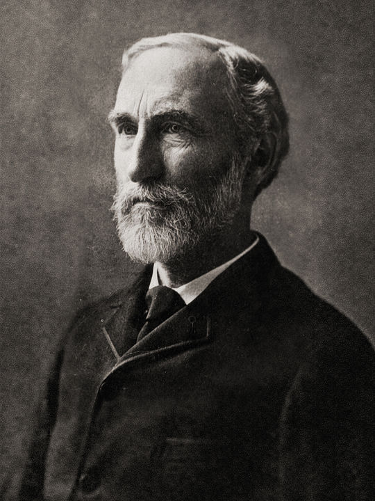
Gibbs' algorithm had an original idea conceived by physicist Josiah Willard Gibbs (figure below), in reference to an analogy between a sampling algorithm and statistical physics (a branch of physics which is based on statistical mechanics). The algorithm was described by brothers Stuart and Donald Geman in 1984 (Geman & Geman, 1984), about eight decades after Gibbs's death.
The Gibbs algorithm is very useful in multidimensional sample spaces (in which there are more than 2 parameters to be sampled for the posterior probability). It is also known as alternating conditional sampling, since we always sample a parameter conditioned to the probability of the other parameters.
The Gibbs algorithm can be seen as a special case of the Metropolis-Hastings algorithm because all proposals are accepted (Gelman, 1992).
Gibbs Algorithm
The essence of Gibbs' algorithm is an iterative sampling of parameters conditioned to other parameters .
Gibbs's algorithm can be described in the following way[6] ( is the parameter, or set of parameters, of interest and is the data):
Define : the prior probability of each of the parameters.
Sample a starting point . We usually sample from a normal distribution or from a distribution specified as the prior distribution of .
For :
Limitations of the Gibbs Algorithm
The main limitation of the Gibbs algorithm is with regard to alternative conditional sampling.
If we compare with the Metropolis algorithm (and consequently Metropolis-Hastings) we have random proposals from a proposal distribution in which we sample each parameter unconditionally to other parameters. In order for the proposals to take us to the posterior probability's correct locations to sample, we have an acceptance/rejection rule for these proposals, otherwise the samples of the Metropolis algorithm would not approach the target distribution of interest. The state changes of the Markov chain are then carried out multidimensionally [7]. As you saw in the Metropolis' figures, in a 2-D space (as is our example's bivariate normal distribution), when there is a change of state in the Markov chain, the new proposal location considers both and , causing diagonal movement in space 2-D sample. In other words, the proposal is done regarding all dimensions of the parameter space.
In the case of the Gibbs algorithm, in our toy example, this movement occurs only in a single parameter, i.e single dimension, as we sample sequentially and conditionally to other parameters. This causes horizontal movements (in the case of ) and vertical movements (in the case of ), but never diagonal movements like the ones we saw in the Metropolis algorithm.
Gibbs – Implementation
Here are some new things compared to the Metropolis algorithm implementation. First to conditionally sample the parameters and , we need to create two new variables β and λ. These variables represent the correlation between and ( and respectively) scaled by the ratio of the variance of and . And then we use these variables in the sampling of and :
function gibbs(
    S::Int64,
    ρ::Float64;
    μ_x::Float64=0.0,
    μ_y::Float64=0.0,
    σ_x::Float64=1.0,
    σ_y::Float64=1.0,
    start_x=-2.5,
    start_y=2.5,
    seed=123,
)
    rgn = MersenneTwister(seed)
    binormal = MvNormal([μ_x; μ_y], [σ_x ρ; ρ σ_y])
    draws = Matrix{Float64}(undef, S, 2)
    x = start_x
    y = start_y
    β = ρ * σ_y / σ_x
    λ = ρ * σ_x / σ_y
    sqrt1mrho2 = sqrt(1 - ρ^2)
    σ_YX = σ_y * sqrt1mrho2
    σ_XY = σ_x * sqrt1mrho2
    @inbounds draws[1, :] = [x y]
    for s in 2:S
        if s % 2 == 0
            y = rand(rgn, Normal(μ_y + β * (x - μ_x), σ_YX))
        else
            x = rand(rgn, Normal(μ_x + λ * (y - μ_y), σ_XY))
        end
        @inbounds draws[s, :] = [x y]
    end
    return draws
end
gibbs (generic function with 1 method)Generally a Gibbs sampler is not implemented in this way. Here I coded the Gibbs algorithm so that it samples a parameter for each iteration. To be more computationally efficient we would sample all parameters are on each iteration. I did it on purpose because I want to show in the animations the real trajectory of the Gibbs sampler in the sample space (vertical and horizontal, not diagonal). So to remedy this I will provide gibbs() double the amount of S (20,000 in total). Also take notice that we are now proposing new parameters' values conditioned on other parameters, so there is not an acceptance/rejection rule here.
X_gibbs = gibbs(S * 2, ρ);As before lets' take a quick peek into X_gibbs, we'll see it's a matrix of and values as columns and the time as rows:
X_gibbs[1:10, :]10×2 Matrix{Float64}:
-2.5 2.5
-2.5 -1.28584
0.200236 -1.28584
0.200236 0.84578
0.952273 0.84578
0.952273 0.523811
0.0202213 0.523811
0.0202213 0.604758
0.438516 0.604758
0.438516 0.515102Again, we construct a Chains object by passing a matrix along with the parameters names as symbols inside the Chains() constructor:
chain_gibbs = Chains(X_gibbs, [:X, :Y]);Then we can get summary statistics regarding our Markov chain derived from the Gibbs algorithm:
summarystats(chain_gibbs)Summary Statistics
parameters mean std mcse ess_bulk ess_tail rhat ess_per_sec
Symbol Float64 Float64 Float64 Float64 Float64 Float64 Missing
X 0.0161 1.0090 0.0217 2152.7581 3985.5939 1.0005 missing
Y 0.0097 1.0071 0.0219 2114.7477 4038.1490 1.0003 missing
Both of X and Y have mean close to 0 and standard deviation close to 1 (which are the theoretical values). Take notice of the ess (effective sample size - ESS) that is around 2,100. Since we used S * 2 as the number of samples, in order for we to compare with Metropolis, we would need to divide the ESS by 2. So our ESS is between 1,000, which is similar to Metropolis' ESS. Now let's calculate the efficiency of our Gibbs algorithm by dividing the ESS by the number of sampling iterations that we've performed also accounting for the S * 2:
(mean(summarystats(chain_gibbs)[:, :ess_tail]) / 2) / S0.20059357221090376Our Gibbs algorithm has around 10.6% efficiency. Which, in my honest opinion, despite the small improvement still sucks...(😂)
Gibbs – Visual Intuition
Oh yes, we have animations for Gibbs also!
The animation in figure below shows the first 100 simulations of the Gibbs algorithm used to generate X_gibbs. Note that all proposals are accepted now, so the at each iteration we sample new parameters values. The blue ellipsis represents the 90% HPD of our toy example's bivariate normal distribution.
f, ax, l = lines(
    getellipsepoints(μ, Σ; confidence=0.9)...;
    label="90% HPD",
    linewidth=2,
    axis=(; limits=(-3, 3, -3, 3), xlabel=L"\theta_1", ylabel=L"\theta_2"),
)
axislegend(ax)
record(f, joinpath(@OUTPUT, "gibbs_anim.gif"); framerate=5) do frame
    for i in 1:200
        scatter!(ax, (X_gibbs[i, 1], X_gibbs[i, 2]); color=(:red, 0.5))
        linesegments!(X_gibbs[i:(i + 1), 1], X_gibbs[i:(i + 1), 2]; color=(:green, 0.5))
        recordframe!(frame)
    end
end;
Now let's take a look how the first 1,000 simulations were, excluding 1,000 initial iterations as warm-up.
f, ax, l = lines(
    getellipsepoints(μ, Σ; confidence=0.9)...;
    label="90% HPD",
    linewidth=2,
    axis=(; limits=(-3, 3, -3, 3), xlabel=L"\theta_1", ylabel=L"\theta_2"),
)
axislegend(ax)
scatter!(
    ax,
    X_gibbs[(2 * warmup):(2 * warmup + 1_000), 1],
    X_gibbs[(2 * warmup):(2 * warmup + 1_000), 2];
    color=(:red, 0.3),
)
And, finally, lets take a look in the all 9,000 samples generated after the warm-up of 1,000 iterations.
f, ax, l = lines(
    getellipsepoints(μ, Σ; confidence=0.9)...;
    label="90% HPD",
    linewidth=2,
    axis=(; limits=(-3, 3, -3, 3), xlabel=L"\theta_1", ylabel=L"\theta_2"),
)
axislegend(ax)
scatter!(ax, X_gibbs[(2 * warmup):end, 1], X_gibbs[(2 * warmup):end, 2]; color=(:red, 0.3))
What happens when we run Markov chains in parallel?
Since the Markov chains are independent, we can run them in parallel. The key to this is defining different starting points for each Markov chain (if you use a sample of a previous distribution of parameters as a starting point this is not a problem). We will use the same toy example of a bivariate normal distribution and that we used in the previous examples, but now with 4 Markov chains in parallel with different starting points[8].
First, let's defined 4 different pairs of starting points using a nice Cartesian product from Julia's Base.Iterators:
const starts = collect(Iterators.product((-2.5, 2.5), (2.5, -2.5)))2×2 Matrix{Tuple{Float64, Float64}}:
(-2.5, 2.5) (-2.5, -2.5)
(2.5, 2.5) (2.5, -2.5)Also, I will restrict this simulation to 100 samples:
const S_parallel = 100;Additionally, note that we are using different seeds:
X_met_1 = metropolis(
    S_parallel, width, ρ; seed=124, start_x=first(starts[1]), start_y=last(starts[1])
);
X_met_2 = metropolis(
    S_parallel, width, ρ; seed=125, start_x=first(starts[2]), start_y=last(starts[2])
);
X_met_3 = metropolis(
    S_parallel, width, ρ; seed=126, start_x=first(starts[3]), start_y=last(starts[3])
);
X_met_4 = metropolis(
    S_parallel, width, ρ; seed=127, start_x=first(starts[4]), start_y=last(starts[4])
);
Acceptance rate is: 0.24
Acceptance rate is: 0.18
Acceptance rate is: 0.18
Acceptance rate is: 0.23
There have been some significant changes in the approval rate for Metropolis proposals. All were around 13%-24%, this is due to the low number of samples (only 100 for each Markov chain), if the samples were larger we would see these values converge to close to 20% according to the previous example of 10,000 samples with a single stream (Roberts et. al, 1997).
Now let's take a look on how those 4 Metropolis Markov chains sample the parameter space starting from different positions. Each chain will have its own marker and path color, so that we can see their different behavior:
using Colors
const logocolors = Colors.JULIA_LOGO_COLORS;
f, ax, l = lines(
    getellipsepoints(μ, Σ; confidence=0.9)...;
    label="90% HPD",
    linewidth=2,
    axis=(; limits=(-3, 3, -3, 3), xlabel=L"\theta_1", ylabel=L"\theta_2"),
)
axislegend(ax)
record(f, joinpath(@OUTPUT, "parallel_met.gif"); framerate=5) do frame
    for i in 1:99
        scatter!(ax, (X_met_1[i, 1], X_met_1[i, 2]); color=(logocolors.blue, 0.5))
        linesegments!(
            X_met_1[i:(i + 1), 1], X_met_1[i:(i + 1), 2]; color=(logocolors.blue, 0.5)
        )
        scatter!(ax, (X_met_2[i, 1], X_met_2[i, 2]); color=(logocolors.red, 0.5))
        linesegments!(
            X_met_2[i:(i + 1), 1], X_met_2[i:(i + 1), 2]; color=(logocolors.red, 0.5)
        )
        scatter!(ax, (X_met_3[i, 1], X_met_3[i, 2]); color=(logocolors.green, 0.5))
        linesegments!(
            X_met_3[i:(i + 1), 1], X_met_3[i:(i + 1), 2]; color=(logocolors.green, 0.5)
        )
        scatter!(ax, (X_met_4[i, 1], X_met_4[i, 2]); color=(logocolors.purple, 0.5))
        linesegments!(
            X_met_4[i:(i + 1), 1], X_met_4[i:(i + 1), 2]; color=(logocolors.purple, 0.5)
        )
        recordframe!(frame)
    end
end;
Now we'll do the the same for Gibbs, taking care to provide also different seeds and starting points:
X_gibbs_1 = gibbs(
    S_parallel * 2, ρ; seed=124, start_x=first(starts[1]), start_y=last(starts[1])
);
X_gibbs_2 = gibbs(
    S_parallel * 2, ρ; seed=125, start_x=first(starts[2]), start_y=last(starts[2])
);
X_gibbs_3 = gibbs(
    S_parallel * 2, ρ; seed=126, start_x=first(starts[3]), start_y=last(starts[3])
);
X_gibbs_4 = gibbs(
    S_parallel * 2, ρ; seed=127, start_x=first(starts[4]), start_y=last(starts[4])
);
Now let's take a look on how those 4 Gibbs Markov chains sample the parameter space starting from different positions. Each chain will have its own marker and path color, so that we can see their different behavior:
f, ax, l = lines(
    getellipsepoints(μ, Σ; confidence=0.9)...;
    label="90% HPD",
    linewidth=2,
    axis=(; limits=(-3, 3, -3, 3), xlabel=L"\theta_1", ylabel=L"\theta_2"),
)
axislegend(ax)
record(f, joinpath(@OUTPUT, "parallel_gibbs.gif"); framerate=5) do frame
    for i in 1:199
        scatter!(ax, (X_gibbs_1[i, 1], X_gibbs_1[i, 2]); color=(logocolors.blue, 0.5))
        linesegments!(
            X_gibbs_1[i:(i + 1), 1], X_gibbs_1[i:(i + 1), 2]; color=(logocolors.blue, 0.5)
        )
        scatter!(ax, (X_gibbs_2[i, 1], X_gibbs_2[i, 2]); color=(logocolors.red, 0.5))
        linesegments!(
            X_gibbs_2[i:(i + 1), 1], X_gibbs_2[i:(i + 1), 2]; color=(logocolors.red, 0.5)
        )
        scatter!(ax, (X_gibbs_3[i, 1], X_gibbs_3[i, 2]); color=(logocolors.green, 0.5))
        linesegments!(
            X_gibbs_3[i:(i + 1), 1], X_gibbs_3[i:(i + 1), 2]; color=(logocolors.green, 0.5)
        )
        scatter!(ax, (X_gibbs_4[i, 1], X_gibbs_4[i, 2]); color=(logocolors.purple, 0.5))
        linesegments!(
            X_gibbs_4[i:(i + 1), 1], X_gibbs_4[i:(i + 1), 2]; color=(logocolors.purple, 0.5)
        )
        recordframe!(frame)
    end
end;
Hamiltonian Monte Carlo – HMC
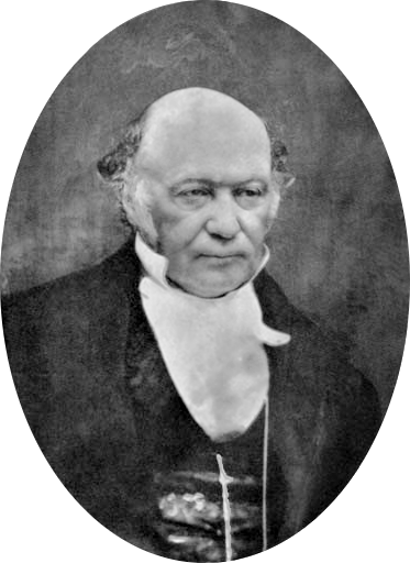
The problems of low acceptance rates of proposals for Metropolis techniques and the low performance of the Gibbs algorithm in multidimensional problems (in which the posterior's topology is quite complex) led to the emergence of a new MCMC technique using Hamiltonian dynamics (in honor of the Irish physicist William Rowan Hamilton (1805-1865) (figure below). The name for this technique is Hamiltonian Monte Carlo – HMC.
The HMC is an adaptation of the Metropolis technique and employs a guided scheme for generating new proposals: this improves the proposal's acceptance rate and, consequently, efficiency. More specifically, the HMC uses the posterior log gradient to direct the Markov chain to regions of higher posterior density, where most samples are collected. As a result, a Markov chain with the well-adjusted HMC algorithm will accept proposals at a much higher rate than the traditional Metropolis algorithm (Roberts et. al, 1997).
HMC was first described in the physics literature (Duane, Kennedy, Pendleton & Roweth, 1987) (which they called the "Hybrid" Monte Carlo – HMC). Soon after, HMC was applied to statistical problems by Neal (1994) (which he called Hamiltonean Monte Carlo – HMC). For an in-depth discussion regarding HMC (which is not the focus of this tutorial), I recommend Neal (2011) and Betancourt (2017).
HMC uses Hamiltonian dynamics applied to particles exploring the topology of a posterior density. In some simulations Metropolis has an acceptance rate of approximately 23%, while HMC 65% (Gelman et al., 2013b). In addition to better exploring the posterior's topology and tolerating complex topologies, HMC is much more efficient than Metropolis and does not suffer from the Gibbs' parameter correlation problem.
For each component , the HMC adds a momentum variable . The subsequent density is increased by an independent distribution of the momentum, thus defining a joint distribution:
HMC uses a proposal distribution that changes depending on the current state in the Markov chain. The HMC discovers the direction in which the posterior distribution increases, called gradient, and distorts the distribution of proposals towards the gradient. In the Metropolis algorithm, the distribution of the proposals would be a (usually) Normal distribution centered on the current position, so that jumps above or below the current position would have the same probability of being proposed. But the HMC generates proposals quite differently.
You can imagine that for high-dimensional posterior densities that have narrow diagonal valleys and even curved valleys, the HMC dynamics will find proposed positions that are much more promising than a naive symmetric proposal distribution, and more promising than the Gibbs sampling, which can get stuck in diagonal walls.
The probability of the Markov chain changing state in the HMC algorithm is defined as:
where is the momentum.
Momentum Distribution –
We normally give a normal multivariate distribution with a mean of 0 and a covariance of , a "mass matrix". To keep things a little bit simpler, we use a diagonal mass matrix . This makes the components of independent with
HMC Algorithm
The HMC algorithm is very similar to the Metropolis algorithm but with the inclusion of the momentum as a way of quantifying the gradient of the posterior distribution:
Sample from a
Simultaneously sample and with leapfrog steps each scaled by a factor. In a leapfrog step, both and are changed, in relation to each other. Repeat the following steps times:
2.1. Use the gradient of log posterior of to produce a half-step of :
2.2 Use the momentum vector to update the parameter vector :
2.3. Use again the gradient of log posterior of to another half-step of :
Assign and as the values of the parameter vector and the momentum vector, respectively, at the beginning of the leapfrog process (step 2) and and as the values after steps. As an acceptance/rejection rule calculate:
Assign:
HMC – Implementation
Alright let's code the HMC algorithm for our toy example's bivariate normal distribution:
using ForwardDiff: gradient
function hmc(
    S::Int64,
    width::Float64,
    ρ::Float64;
    L=40,
    ϵ=0.001,
    μ_x::Float64=0.0,
    μ_y::Float64=0.0,
    σ_x::Float64=1.0,
    σ_y::Float64=1.0,
    start_x=-2.5,
    start_y=2.5,
    seed=123,
)
    rgn = MersenneTwister(seed)
    binormal = MvNormal([μ_x; μ_y], [σ_x ρ; ρ σ_y])
    draws = Matrix{Float64}(undef, S, 2)
    accepted = 0::Int64
    x = start_x
    y = start_y
    @inbounds draws[1, :] = [x y]
    M = [1.0 0.0; 0.0 1.0]
    ϕ_d = MvNormal([0.0, 0.0], M)
    for s in 2:S
        x_ = rand(rgn, Uniform(x - width, x + width))
        y_ = rand(rgn, Uniform(y - width, y + width))
        ϕ = rand(rgn, ϕ_d)
        kinetic = sum(ϕ .^ 2) / 2
        log_p = logpdf(binormal, [x, y]) - kinetic
        ϕ += 0.5 * ϵ * gradient(x -> logpdf(binormal, x), [x_, y_])
        for l in 1:L
            x_, y_ = [x_, y_] + (ϵ * M * ϕ)
            ϕ += +0.5 * ϵ * gradient(x -> logpdf(binormal, x), [x_, y_])
        end
        ϕ = -ϕ # make the proposal symmetric
        kinetic = sum(ϕ .^ 2) / 2
        log_p_ = logpdf(binormal, [x_, y_]) - kinetic
        r = exp(log_p_ - log_p)

        if r > rand(rgn, Uniform())
            x = x_
            y = y_
            accepted += 1
        end
        @inbounds draws[s, :] = [x y]
    end
    println("Acceptance rate is: $(accepted / S)")
    return draws
end
hmc (generic function with 1 method)In the hmc() function above I am using the gradient() function from ForwardDiff.jl (Revels, Lubin & Papamarkou, 2016) which is Julia's package for forward mode auto differentiation (autodiff). The gradient() function accepts a function as input and an array . It literally evaluates the function at and returns the gradient . This is one the advantages of Julia: I don't need to implement an autodiff for logpdf()s of any distribution, it will be done automatically for any one from Distributions.jl. You can also try reverse mode autodiff with ReverseDiff.jl if you want to; and it will also very easy to get a gradient. Now, we've got carried away with Julia's amazing autodiff potential... Let me show you an example of a gradient of a log PDF evaluated at some value. I will use our mvnormal bivariate normal distribution as an example and evaluate its gradient at and :
gradient(x -> logpdf(mvnormal, x), [1, -1])2-element Vector{Float64}:
-5.000000000000003
5.000000000000003So the gradient tells me that the partial derivative of with respect to our mvnormal distribution is -5 and the partial derivative of with respect to our mvnormal distribution is 5.
Now let's run our HMC Markov chain. We are going to use and (don't ask me how I found out) :
X_hmc = hmc(S, width, ρ; ϵ=0.0856, L=40);Acceptance rate is: 0.2079
Our acceptance rate is 20.79%. As before lets' take a quick peek into X_hmc, we'll see it's a matrix of and values as columns and the time as rows:
X_hmc[1:10, :]10×2 Matrix{Float64}:
-2.5 2.5
-2.5 2.5
-1.50904 1.52822
-1.50904 1.52822
-1.85829 -0.464346
-0.739967 -1.15873
-0.739967 -1.15873
-0.739967 -1.15873
-0.739967 -1.15873
-0.739967 -1.15873Again, we construct a Chains object by passing a matrix along with the parameters names as symbols inside the Chains() constructor:
chain_hmc = Chains(X_hmc, [:X, :Y]);Then we can get summary statistics regarding our Markov chain derived from the HMC algorithm:
summarystats(chain_hmc)Summary Statistics
parameters mean std mcse ess_bulk ess_tail rhat ess_per_sec
Symbol Float64 Float64 Float64 Float64 Float64 Float64 Missing
X 0.0169 0.9373 0.0222 1738.2585 1537.0420 1.0014 missing
Y 0.0073 0.9475 0.0237 1556.0589 1640.5275 1.0003 missing
Both of X and Y have mean close to 0 and standard deviation close to 1 (which are the theoretical values). Take notice of the ess (effective sample size - ESS) that is around 1,600. Now let's calculate the efficiency of our HMC algorithm by dividing the ESS by the number of sampling iterations:
mean(summarystats(chain_hmc)[:, :ess_tail]) / S0.15887847790933807We see that a simple naïve (and not well-calibrated[9]) HMC has 70% more efficiency from both Gibbs and Metropolis. ≈ 10% versus ≈ 17%. Great! 😀
HMC – Visual Intuition
This wouldn't be complete without animations for HMC!
The animation in figure below shows the first 100 simulations of the HMC algorithm used to generate X_hmc. Note that we have a gradient-guided proposal at each iteration, so the animation would resemble more like a very lucky random-walk Metropolis [10]. The blue ellipsis represents the 90% HPD of our toy example's bivariate normal distribution.
f, ax, l = lines(
    getellipsepoints(μ, Σ; confidence=0.9)...;
    label="90% HPD",
    linewidth=2,
    axis=(; limits=(-3, 3, -3, 3), xlabel=L"\theta_1", ylabel=L"\theta_2"),
)
axislegend(ax)
record(f, joinpath(@OUTPUT, "hmc_anim.gif"); framerate=5) do frame
    for i in 1:100
        scatter!(ax, (X_hmc[i, 1], X_hmc[i, 2]); color=(:red, 0.5))
        linesegments!(X_hmc[i:(i + 1), 1], X_hmc[i:(i + 1), 2]; color=(:green, 0.5))
        recordframe!(frame)
    end
end;
As usual, let's take a look how the first 1,000 simulations were, excluding 1,000 initial iterations as warm-up.
f, ax, l = lines(
    getellipsepoints(μ, Σ; confidence=0.9)...;
    label="90% HPD",
    linewidth=2,
    axis=(; limits=(-3, 3, -3, 3), xlabel=L"\theta_1", ylabel=L"\theta_2"),
)
axislegend(ax)
scatter!(
    ax,
    X_hmc[warmup:(warmup + 1_000), 1],
    X_hmc[warmup:(warmup + 1_000), 2];
    color=(:red, 0.3),
)
And, finally, lets take a look in the all 9,000 samples generated after the warm-up of 1,000 iterations.
f, ax, l = lines(
    getellipsepoints(μ, Σ; confidence=0.9)...;
    label="90% HPD",
    linewidth=2,
    axis=(; limits=(-3, 3, -3, 3), xlabel=L"\theta_1", ylabel=L"\theta_2"),
)
axislegend(ax)
scatter!(ax, X_hmc[warmup:end, 1], X_hmc[warmup:end, 2]; color=(:red, 0.3))
HMC – Complex Topologies
There are cases where HMC will be much better than Metropolis or Gibbs. In particular, these cases focus on complicated and difficult-to-explore posterior topologies. In these contexts, an algorithm that can guide the proposals to regions of higher density (such as the case of the HMC) is able to explore much more efficient (less iterations for convergence) and effective (higher rate of acceptance of the proposals).
See figure below for an example of a bimodal posterior density with also the marginal histogram of and :
d1 = MvNormal([10, 2], [1 0; 0 1])
d2 = MvNormal([0, 0], [8.4 2.0; 2.0 1.7])

d = MixtureModel([d1, d2])

x = -6:0.01:15
y = -2.5:0.01:4.2
dens_mixture = [pdf(d, [i, j]) for i in x, j in y]

f, ax, s = surface(
    x,
    y,
    dens_mixture;
    axis=(type=Axis3, xlabel=L"X", ylabel=L"Y", zlabel="PDF", azimuth=pi / 4),
)
And to finish an example of Neal's funnel (Neal, 2003) in the figure below. This is a very difficult posterior to be sampled even for HMC, as it varies in geometry in the dimensions and . This means that the HMC sampler has to change the leapfrog steps and the scaling factor every time, since at the top of the image (the top of the funnel) a large value of is needed along with a small ; and at the bottom (at the bottom of the funnel) the opposite: small and large .
funnel_y = rand(Normal(0, 3), 10_000)
funnel_x = rand(Normal(), 10_000) .* exp.(funnel_y / 2)

f, ax, s = scatter(
    funnel_x,
    funnel_y;
    color=(:steelblue, 0.3),
    axis=(; xlabel=L"X", ylabel=L"Y", limits=(-100, 100, nothing, nothing)),
)
"I understood nothing..."
If you haven't understood anything by now, don't despair. Skip all the formulas and get the visual intuition of the algorithms. See the limitations of Metropolis and Gibbs and compare the animations and figures with those of the HMC. The superiority of efficiency (more samples with low autocorrelation - ESS) and effectiveness (more samples close to the most likely areas of the target distribution) is self-explanatory by the images.
In addition, you will probably never have to code your HMC algorithm (Gibbs, Metropolis or any other MCMC) by hand. For that there are packages like Turing's AdvancedHMC.jl In addition, AdvancedHMC has a modified HMC with a technique called No-U-Turn Sampling (NUTS)[11] (Hoffman & Gelman, 2011) that selects automatically the values of (scaling factor) and (leapfrog steps). The performance of the HMC is highly sensitive to these two "hyperparameters" (parameters that must be specified by the user). In particular, if is too small, the algorithm exhibits undesirable behavior of a random walk, while if is too large, the algorithm wastes computational efficiency. NUTS uses a recursive algorithm to build a set of likely candidate points that span a wide range of proposal distribution, automatically stopping when it starts to go back and retrace its steps (why it doesn't turn around - No U-turn), in addition NUTS also automatically calibrates simultaneously and .
MCMC Metrics
All Markov chains have some convergence and diagnostics metrics that you should be aware of. Note that this is still an ongoing area of intense research and new metrics are constantly being proposed (e.g. Lambert & Vehtari (2020) or Vehtari, Gelman., Simpson, Carpenter & Bürkner (2021)) To show MCMC metrics let me recover our six-sided dice example from 4. How to use Turing:
using Turing

@model function dice_throw(y)
    #Our prior belief about the probability of each result in a six-sided dice.
    #p is a vector of length 6 each with probability p that sums up to 1.
    p ~ Dirichlet(6, 1)

    #Each outcome of the six-sided dice has a probability p.
    return y ~ filldist(Categorical(p), length(y))
end;
Let's once again generate 1,000 throws of a six-sided dice:
data_dice = rand(DiscreteUniform(1, 6), 1_000);Like before we'll sample using NUTS() and 1,000 iterations. Note that you can use Metropolis with MH(), Gibbs with Gibbs() and HMC with HMC() if you want to. You can check all Turing's different MCMC samplers in Turing's documentation.
model = dice_throw(data_dice)
chain = sample(model, NUTS(), 1_000);
summarystats(chain)
Summary Statistics
parameters mean std mcse ess_bulk ess_tail rhat ess_per_sec
Symbol Float64 Float64 Float64 Float64 Float64 Float64 Float64
p[1] 0.1689 0.0118 0.0003 1965.3374 876.7033 0.9995 613.7843
p[2] 0.1661 0.0119 0.0003 1419.7589 739.3257 1.0001 443.3975
p[3] 0.1600 0.0108 0.0003 1594.9950 873.7550 0.9990 498.1246
p[4] 0.1700 0.0116 0.0003 1998.9151 884.6355 1.0045 624.2708
p[5] 0.1710 0.0117 0.0003 1670.1179 813.8896 0.9994 521.5858
p[6] 0.1641 0.0120 0.0003 2055.8182 792.1886 1.0011 642.0419
We have the following columns that outputs some kind of MCMC summary statistics:
mcse: Monte Carlo Standard Error, the uncertainty about a statistic in the sample due to sampling error.ess: Effective Sample Size, a rough approximation of the number of effective samples sampled by the MCMC estimated by the value ofrhat.rhat: a metric of convergence and stability of the Markov chain.
The most important metric to take into account is the rhat which is a metric that measures whether the Markov chains are stable and converged to a value during the total progress of the sampling procedure. It is basically the proportion of variation when comparing two halves of the chains after discarding the warmups. A value of 1 implies convergence and stability. By default, rhat must be less than 1.01 for the Bayesian estimation to be valid (Brooks & Gelman, 1998; Gelman & Rubin, 1992).
Note that all of our model's parameters have achieve a nice ess and, more important, rhat in the desired range, a solid indicator that the Markov chain is stable and has converged to the estimated parameter values.
What looks like when your model doesn't converge
Depending on the model and data, it is possible that HMC (even with NUTS) will not achieve convergence. NUTS will not converge if it encounters divergences either due to a very pathological posterior density topology or if you supply improper parameters. To exemplify let me run a "bad" chain by passing the NUTS() constructor a target acceptance rate of 0.3 with only 500 sampling iterations (including warmup of 1,000 iters):
bad_chain = sample(model, NUTS(0.3), 500)
summarystats(bad_chain)
Summary Statistics
parameters mean std mcse ess_bulk ess_tail rhat ess_per_sec
Symbol Float64 Float64 Float64 Float64 Float64 Float64 Float64
p[1] 0.1684 0.0098 0.0029 8.6088 16.0774 1.1119 128.4895
p[2] 0.1657 0.0130 0.0029 12.6348 NaN 1.0553 188.5793
p[3] 0.1637 0.0112 0.0025 20.4216 26.6760 1.2401 304.7994
p[4] 0.1719 0.0102 0.0022 27.0245 23.5726 1.0613 403.3510
p[5] 0.1728 0.0181 0.0056 13.6728 13.2203 1.1900 204.0718
p[6] 0.1575 0.0175 0.0059 6.4771 3.5114 1.1389 96.6725
Here we can see that the ess and rhat of the bad_chain are really bad! There will be several divergences that we can access in the column numerical_error of a Chains object. Here we have 64 divergences.
sum(bad_chain[:numerical_error])17.0Also we can see the Markov chain acceptance rate in the column acceptance_rate. This is the bad_chain acceptance rate:
mean(bad_chain[:acceptance_rate])0.018655899447476025And now the "good" chain:
mean(chain[:acceptance_rate])0.7934378228300696What a difference huh? 80% versus 1.5%.
MCMC Visualizations
Besides the rhat values, we can also visualize the Markov chain with a traceplot. The traceplot is the overlap of the MCMC chain sampling for each estimated parameter (vertical axis). The idea is that the chains mix and that there is no slope or visual pattern along the iterations (horizontal axis). This demonstrates that the chains have mixed converged to a certain value of the parameter and remained in that region during a good part (or all) of the Markov chain sampling. We can do that with the MCMCChains.jl's function traceplot(). Let's look the "good" chain first:
using AlgebraOfGraphics
params = names(chain, :parameters)
chain_mapping =
    mapping(params .=> "sample value") *
    mapping(; color=:chain => nonnumeric, row=dims(1) => renamer(params))
plt = data(chain) * mapping(:iteration) * chain_mapping * visual(Lines)
f = Figure(; resolution=(1200, 900))
draw!(f[1, 1], plt)
chainAnd now the bad_chain:
params = names(bad_chain, :parameters)
chain_mapping =
    mapping(params .=> "sample value") *
    mapping(; color=:chain => nonnumeric, row=dims(1) => renamer(params))
plt = data(bad_chain) * mapping(:iteration) * chain_mapping * visual(Lines)
f = Figure(; resolution=(1200, 900))
draw!(f[1, 1], plt)
bad_chainWe can see that the bad_chain is all over the place and has definitely not converged or became stable.
How to make your Markov chains converge
First: Before making fine adjustments to the number of chains or the number of iterations (among others ...) know that Turing's NUTS sampler is very efficient and effective in exploring the most diverse and complex "crazy" topologies of posteriors' target distributions. The standard arguments NUTS() work perfectly for 99% of cases (even in complex models). That said, most of the time when you have sampling and computational problems in your Bayesian model, the problem is in the model specification and not in the MCMC sampling algorithm. This is known as Folk Theorem (Gelman, 2008). In the words of Andrew Gelman:
"When you have computational problems, often there's a problem with your model".
Andrew Gelman (Gelman, 2008)
If your Bayesian model has problems with convergence there are some steps that can be tried[12]. Listed here from the simplest to the most complex:
Increase the number of iterations and chains: First option is to increase the number of MCMC iterations and it is also possible to increase the number of parallel chains to be sampled.
Model reparameterization: the second option is to reparameterize the model. There are two ways to parameterize the model: the first with centered parameterization (CP) and the second with non-centered parameterization (NCP). NCP is most useful in Multilevel Models, therefore we will cover NCP in 10. Multilevel Models.
Collect more data: sometimes the model is too complex and we need a larger sample to get stable estimates.
Rethink the model: convergence failure when we have adequate sampling is usually due to a specification of priors and likelihood function that are not compatible with the data. In this case, it is necessary to rethink the data's generative process in which the model's assumptions are anchored.
Footnotes
| [1] | the symbol (\propto) should be read as "proportional to".
|
| [2] | some references call this process burnin. |
| [3] | if you want a better explanation of the Metropolis and Metropolis-Hastings algorithms I suggest to see Chib & Greenberg (1995). |
| [4] | Due to easier computational complexity and to avoid numeric overflow we generally use sum of logs instead of multiplications, specially when dealing with probabilities, i.e. . |
| [5] | this is one of the packages of Turing's ecosystem. I recommend you to take a look into 4. How to use Turing. |
| [6] | if you want a better explanation of the Gibbs algorithm I suggest to see Casella & George (1992). |
| [7] | this will be clear in the animations and images. |
| [8] | note that there is some shenanigans here to take care. You would also want to have different seeds for the random number generator in each Markov chain. This is why metropolis() and gibbs() have a seed parameter.
|
| [9] | as detailed in the following sections, HMC is quite sensitive to the choice of and and I haven't tried to get the best possible combination of those. |
| [10] | or a not-drunk random-walk Metropolis 😂. |
| [11] | NUTS is an algorithm that uses the symplectic leapfrog integrator and builds a binary tree composed of leaf nodes that are simulations of Hamiltonian dynamics using leapfrog steps in forward or backward directions in time where is the integer representing the iterations of the construction of the binary tree. Once the simulated particle starts to retrace its trajectory, the tree construction is interrupted and the ideal number of leapfrog steps is defined as in time from the beginning of the retrogression of the trajectory. So the simulated particle never "turns around" so "No U-turn". For more details on the algorithm and how it relates to Hamiltonian dynamics see Hoffman & Gelman (2011). |
| [12] | furthermore, if you have high-correlated variables in your model, you can try a QR decomposition of the data matrix . I will cover QR decomposition and other Turing's computational "tricks of the trade" in 11. Computational Tricks with Turing. |
References
Betancourt, M. (2017, January 9). A Conceptual Introduction to Hamiltonian Monte Carlo. Retrieved November 6, 2019, from http://arxiv.org/abs/1701.02434
Brooks, S., Gelman, A., Jones, G., & Meng, X.-L. (2011). Handbook of Markov Chain Monte Carlo. Retrieved from https://books.google.com?id=qfRsAIKZ4rIC
Brooks, S. P., & Gelman, A. (1998). General Methods for Monitoring Convergence of Iterative Simulations. Journal of Computational and Graphical Statistics, 7(4), 434–455. https://doi.org/10.1080/10618600.1998.10474787
Casella, G., & George, E. I. (1992). Explaining the gibbs sampler. The American Statistician, 46(3), 167–174. https://doi.org/10.1080/00031305.1992.10475878
Chib, S., & Greenberg, E. (1995). Understanding the Metropolis-Hastings Algorithm. The American Statistician, 49(4), 327–335. https://doi.org/10.1080/00031305.1995.10476177
Duane, S., Kennedy, A. D., Pendleton, B. J., & Roweth, D. (1987). Hybrid Monte Carlo. Physics Letters B, 195(2), 216–222. https://doi.org/10.1016/0370-2693(87)91197-X
Eckhardt, R. (1987). Stan Ulam, John von Neumann, and the Monte Carlo Method. Los Alamos Science, 15(30), 131–136.
Gelman, A. (1992). Iterative and Non-Iterative Simulation Algorithms. Computing Science and Statistics (Interface Proceedings), 24, 457–511. PROCEEDINGS PUBLISHED BY VARIOUS PUBLISHERS.
Gelman, A. (2008). The folk theorem of statistical computing. Retrieved from https://statmodeling.stat.columbia.edu/2008/05/13/thefolktheore/
Gelman, A., Carlin, J. B., Stern, H. S., Dunson, D. B., Vehtari, A., & Rubin, D. B. (2013a). Basics of Markov Chain Simulation. In Bayesian Data Analysis. Chapman and Hall/CRC.
Gelman, A., Carlin, J. B., Stern, H. S., Dunson, D. B., Vehtari, A., & Rubin, D. B. (2013b). Bayesian Data Analysis. Chapman and Hall/CRC.
Gelman, A., & Rubin, D. B. (1992). Inference from Iterative Simulation Using Multiple Sequences. Statistical Science, 7(4), 457–472. https://doi.org/10.1214/ss/1177011136
Geman, S., & Geman, D. (1984). Stochastic Relaxation, Gibbs Distributions, and the Bayesian Restoration of Images. IEEE Transactions on Pattern Analysis and Machine Intelligence, PAMI-6(6), 721–741. https://doi.org/10.1109/TPAMI.1984.4767596
Hastings, W. K. (1970). Monte Carlo sampling methods using Markov chains and their applications. Biometrika, 57(1), 97–109. https://doi.org/10.1093/biomet/57.1.97
Hoffman, M. D., & Gelman, A. (2011). The No-U-Turn Sampler: Adaptively Setting Path Lengths in Hamiltonian Monte Carlo. Journal of Machine Learning Research, 15(1), 1593–1623. Retrieved from http://arxiv.org/abs/1111.4246
Lambert, B., & Vehtari, A. (2020). : A robust MCMC convergence diagnostic with uncertainty using decision tree classifiers. ArXiv:2003.07900 [Stat]. http://arxiv.org/abs/2003.07900
Metropolis, N., Rosenbluth, A. W., Rosenbluth, M. N., Teller, A. H., & Teller, E. (1953). Equation of State Calculations by Fast Computing Machines. The Journal of Chemical Physics, 21(6), 1087–1092. https://doi.org/10.1063/1.1699114
Neal, Radford M. (1994). An Improved Acceptance Procedure for the Hybrid Monte Carlo Algorithm. Journal of Computational Physics, 111(1), 194–203. https://doi.org/10.1006/jcph.1994.1054
Neal, Radford M. (2003). Slice Sampling. The Annals of Statistics, 31(3), 705–741. Retrieved from https://www.jstor.org/stable/3448413
Neal, Radford M. (2011). MCMC using Hamiltonian dynamics. In S. Brooks, A. Gelman, G. L. Jones, & X.-L. Meng (Eds.), Handbook of markov chain monte carlo.
Revels, J., Lubin, M., & Papamarkou, T. (2016). Forward-Mode Automatic Differentiation in Julia. ArXiv:1607.07892 [Cs]. http://arxiv.org/abs/1607.07892
Roberts, G. O., Gelman, A., & Gilks, W. R. (1997). Weak convergence and optimal scaling of random walk Metropolis algorithms. Annals of Applied Probability, 7(1), 110–120. https://doi.org/10.1214/aoap/1034625254
Vehtari, A., Gelman, A., Simpson, D., Carpenter, B., & Bürkner, P.-C. (2021). Rank-Normalization, Folding, and Localization: An Improved Rˆ for Assessing Convergence of MCMC. Bayesian Analysis, 1(1), 1–28. https://doi.org/10.1214/20-BA1221